Try it on your own data
Every report in this article is in the free plan. One snippet for web and apps, up to 10 sites.
Start freeScatter plots are the quickest way to see whether two numbers move together, and the quickest way to fool yourself if you skip the details. This guide covers when to use one, a five-pass method for reading it, and a worked example with 12 landing pages where load time and conversion correlate at −0.91, until one extra page drops it to −0.39.
What you will learn
- Use a scatter plot for paired numeric values across many items
- Read direction, form, strength, outliers and clusters in that order
- Pearson r measures linear strength only; always look at the plot
- One outlier from a different population can flip the conclusion
- Correlation in a scatter plot is not causation; check confounders
What is a scatter plot?
A scatter plot (also scatter chart or scatter graph) shows the relationship between two numeric variables. Each observation is one dot: its position on the horizontal x-axis is one value, its position on the vertical y-axis is the other. Looking at the cloud of dots tells you whether the two variables move together, how strongly, in what shape, and which observations do not follow the crowd.
Line charts show one variable over time. Bar charts compare categories. Scatter plots answer a different question: when this goes up, what happens to that?
When to use a scatter plot
| Question | Example in analytics | Scatter plot? |
|---|---|---|
| Do two measures move together? | Page load time vs conversion rate, per page | Yes |
| Are there distinct groups? | Sessions vs revenue per customer: casual vs power users | Yes |
| Which items are unusual? | Campaigns with high spend but low sign-ups | Yes |
| How does one value change over time? | Daily sessions | No, use a line chart |
| Which category is biggest? | Traffic by channel | No, use a bar chart |
| Shares of a whole | Device mix | No, use a bar or stacked bar |
Use it when you have paired numeric values for many items (pages, campaigns, customers, days) and want to see the relationship before you calculate anything.
| Chart | Best for | Analytics example |
|---|---|---|
| Scatter plot | Relationship between two numbers | LCP vs conversion per page |
| Line chart | Change over time | Daily sessions |
| Bar chart | Comparing categories | Sessions by channel |
| Bubble chart | Two numbers plus a size | Spend vs sign-ups, sized by traffic |
Pick the chart by the question, not by the data you have.
How to read a scatter plot
Read it in five passes:
- Direction. Dots rising from left to right: a positive relationship. Falling: negative. No slope: none.
- Form. Do the dots follow a straight line, a curve, or flatten out after a point? Many web metrics have diminishing returns: conversion improves quickly as load time drops from 5 to 3 seconds, then barely moves below 2.
- Strength. A tight band means a strong relationship; a loose cloud, a weak one. The Pearson correlation coefficient r puts a number on linear strength, from −1 to +1.
- Outliers. Points far from the pattern. They are either errors to fix or the most interesting stories in the chart; see outliers in data.
- Clusters. Separate clouds usually mean a hidden third variable, such as device type or plan, that should be split out.
As a rough guide for |r|: below 0.3 is weak, 0.3 to 0.7 moderate, above 0.7 strong. But always look at the plot: very different patterns can share the same r, which is the point of Anscombe's famous four datasets.
Worked example: page speed vs conversion
We took 12 landing pages on a B2B site and plotted each page's 75th-percentile Largest Contentful Paint on the x-axis against its visit-to-sign-up conversion rate on the y-axis (sample data):
| Page | LCP P75 (s) | Conversion (%) |
|---|---|---|
| /pricing | 1.4 | 4.8 |
| /demo | 1.7 | 4.1 |
| /signup | 1.9 | 4.6 |
| /features | 2.1 | 3.8 |
| /integrations | 2.3 | 4.3 |
| /compare | 2.4 | 3.6 |
| /use-cases | 2.6 | 4 |
| /templates | 2.9 | 3.1 |
| /customers | 3.1 | 3.7 |
| /partners | 3.4 | 3.2 |
| /webinars | 3.8 | 2.6 |
| /resources | 4.6 | 2.5 |
What the plot shows: the dots fall from upper left to lower right. Faster pages convert better.
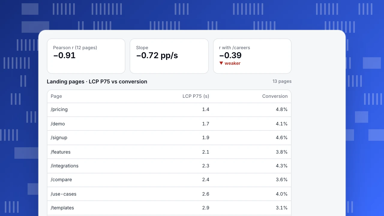
The numbers: the mean LCP is 2.68 s and mean conversion 3.69%. Pearson r = −0.91, so the linear relationship is strong. A least-squares trend line through the dots has a slope of −0.72: each extra second of LCP goes with about 0.72 percentage points less conversion, and r² = 0.83 means load time accounts for most of the variation between these pages.
Now add one more page. The careers page loads in 1.6 s but converts at 1.2%, because almost nobody visits it to sign up. With it included, r drops to −0.39 and the slope to −0.41. One point changed the conclusion from "strong" to "moderate". The fix is not to delete it silently: it belongs to a different population (non-commercial pages) and should be plotted in a different color or excluded with a stated rule.
What the plot does not show: causation. Slow pages here are also the long content pages (resources, webinars) that attract early-stage readers who convert less anyway. Page type is a confounding variable. To know whether speed itself moves conversion, speed up a few pages and compare against similar pages you did not change. See correlation vs causation.
Pearson r (12 pages)
−0.91
Slope
−0.72 pp/s
r with /careers
−0.39
▼ weaker
Landing pages · LCP P75 vs conversion
13 pages| Page | LCP P75 (s) | Conversion |
|---|---|---|
| /pricing | 1.4 | 4.8% |
| /demo | 1.7 | 4.1% |
| /signup | 1.9 | 4.6% |
| /features | 2.1 | 3.8% |
| /integrations | 2.3 | 4.3% |
| /compare | 2.4 | 3.6% |
| /use-cases | 2.6 | 4.0% |
| /templates | 2.9 | 3.1% |
| /customers | 3.1 | 3.7% |
| /partners | 3.4 | 3.2% |
| /webinars | 3.8 | 2.6% |
| /resources | 4.6 | 2.5% |
| /careers | 1.6 | 1.2% |
Highlighted row: the /careers outlier.
How to make a good scatter plot
- Put the presumed cause on the x-axis and the outcome on the y-axis.
- Start axes where the data is, not at zero, unless zero is meaningful. Label units.
- Handle overplotting. With thousands of points, use transparency, smaller dots, jitter, or switch to a binned heatmap.
- Use log scales for skewed data such as revenue per customer or pageviews per page, where a few items are 100× the rest.
- Encode a third variable carefully. Color for a category (device, plan) works; size for a number (traffic) works as a bubble chart but is hard to read precisely.
- Add a trend line only if the form is roughly linear. A straight line through a curve misleads.
- Show the sample size and the time period in the caption.
Common mistakes
- Reading correlation as causation. The most common misuse, especially with confounders like page type, season or channel.
- Mixing populations. Combining mobile and desktop, or new and returning users, can hide or reverse a relationship (Simpson's paradox).
- Ignoring small samples. Five points can show an impressive r by chance.
- Plotting time series against each other. Two metrics that both grew over a year will correlate, even if unrelated. Compare changes, not levels.
- Using averages that hide distribution. Plot P75 or median for skewed measures like load time.
Scatter plots with TapCub data
TapCub reports page-level performance (LCP, INP, CLS at P75) and page-level conversions to goals. To build the chart above, pull both numbers per page with SQL queries or a CSV export, then plot them in a spreadsheet or notebook. Read Core Web Vitals first to choose the right percentile. If the relationship looks strong, test it: improve two or three slow pages and compare their conversion trend with similar pages you left alone.
See also: Anscombe's quartet.
Sources
- NIST/SEMATECH. e-Handbook: scatter plot and correlation.
- Anscombe, F. J. (1973). Graphs in statistical analysis. The American Statistician, 27(1), 17–21.
- Cleveland, W. S. (1994). The Elements of Graphing Data. Hobart Press.
Was this article helpful?
We use your answers to fix and expand this page.
Couldn’t send. Please try again in a minute.
Thanks for the feedback. We’ll use it to improve this page.You’ve already sent feedback on this page. Thanks.

Product Experience Specialist
Writes about product experience, practical workflows, and growth, turning complex processes into clear steps for everyday decisions.