Try it on your own data
Every report in this article is in the free plan. One snippet for web and apps, up to 10 sites.
Start freeRegression turns a scatter of points into numbers you can budget with: how much the outcome moves per unit of each driver, and how sure you can be. This guide walks through 12 weeks of ad spend, organic traffic and sign-ups, where a one-variable model credits ads with 14 sign-ups per $1,000 and a model that controls for organic demand says 10.6.
What you will learn
- Regression estimates effect size, uncertainty and predictions
- Omitting a correlated driver biases coefficients
- Use adjusted R² to compare models with different predictors
- Check linearity, independence, normality and equal variance
- Coefficients from observational data are associations, not causes
What is regression analysis?
Regression analysis is a family of statistical methods that estimate how an outcome (the dependent variable) changes when one or more inputs (the independent variables or predictors) change. It gives you three things a chart alone cannot: the size of each relationship, how uncertain that size is, and a way to predict the outcome for new values.
In analytics, typical questions are: how many extra sign-ups come with each extra $1,000 of ad spend, holding organic traffic constant? How much does each second of load time cost in conversion? Which customer behaviors predict churn?
The simplest form is a line through a scatter plot:
y = β₀ + β₁x + ε
where β₀ is the intercept, β₁ the slope (change in y per one-unit change in x), and ε the error the line does not explain. Ordinary least squares (OLS) picks the line that minimizes the sum of squared errors.
Types of regression
| Type | Outcome | Analytics example |
|---|---|---|
| Simple linear | Continuous, one predictor | Sign-ups vs ad spend |
| Multiple linear | Continuous, several predictors | Sign-ups vs spend, organic traffic, holidays |
| Logistic | Yes / no | Will this trial convert? Will this account churn? |
| Poisson / negative binomial | Counts | Support tickets per account per month |
| Polynomial / spline | Curved relationships | Conversion vs load time with diminishing returns |
| Regression with time terms | Time series | Weekly sales with trend and seasonality |
| Type | Outcome | Example |
|---|---|---|
| Simple linear | Continuous, one predictor | Sign-ups vs spend |
| Multiple linear | Continuous, several predictors | Sign-ups vs spend and organic |
| Logistic | Yes / no | Will a trial convert? |
| Poisson | Counts | Tickets per account |
Choose the type by the outcome you are modeling.
Worked example: does ad spend drive sign-ups?
Twelve weeks of data for a SaaS site (sample data): weekly paid spend in thousands of dollars, organic sessions in thousands, and sign-ups.
| Week | Ad spend ($k) | Organic sessions (k) | Sign-ups |
|---|---|---|---|
| 1 | 2.0 | 8.0 | 109 |
| 2 | 2.5 | 9.6 | 116 |
| 3 | 3.0 | 8.6 | 121 |
| 4 | 2.2 | 10.4 | 121 |
| 5 | 3.5 | 9.0 | 131 |
| 6 | 4.0 | 11.2 | 140 |
| 7 | 3.2 | 10.8 | 135 |
| 8 | 4.5 | 10.0 | 139 |
| 9 | 5.0 | 12.2 | 162 |
| 10 | 4.2 | 11.6 | 142 |
| 11 | 5.5 | 11.0 | 158 |
| 12 | 6.0 | 12.8 | 170 |
Model 1: sign-ups on spend only
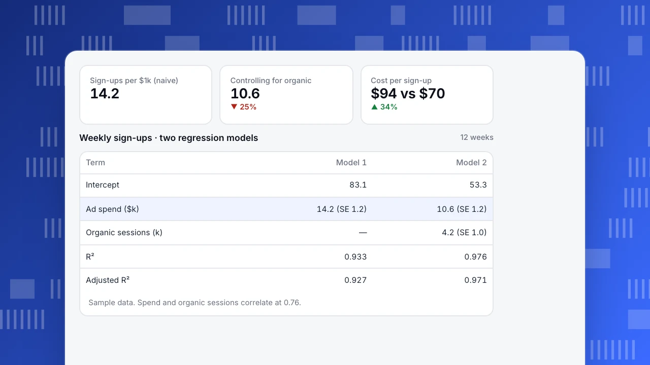
Sign-ups = 83.1 + 14.2 × spend. Standard error of the slope 1.2, R² = 0.93.
Read naively: each extra $1,000 brings 14 sign-ups, so a sign-up costs about $70.
Model 2: add organic sessions
Sign-ups = 53.3 + 10.6 × spend + 4.2 × organic sessions (k). Standard errors 1.2 and 1.0, R² = 0.976, adjusted R² = 0.971.
The spend coefficient fell by a quarter. Why? Spend and organic traffic rose together over the quarter (their correlation is 0.76) because the team spent more during the busy season, when organic interest was also high. Model 1 credited spend with sign-ups that came from seasonal organic demand. Organic traffic was a confounding variable, and leaving it out biased the estimate upward. That is omitted variable bias.
Holding organic sessions constant, an extra $1,000 goes with about 10.6 sign-ups: cost per sign-up closer to $94 than $70, a difference that changes a budget decision.
Prediction: for a week with $5,000 spend and 11,000 organic sessions, Model 2 predicts 53.3 + 53.0 + 45.8 ≈ 152 sign-ups. The residual standard error is about 3 sign-ups, so a week far outside that range is worth investigating.
Sign-ups per $1k (naive)
14.2
Controlling for organic
10.6
▼ 25%
Cost per sign-up
$94 vs $70
▲ 34%
Weekly sign-ups · two regression models
12 weeks| Term | Model 1 | Model 2 |
|---|---|---|
| Intercept | 83.1 | 53.3 |
| Ad spend ($k) | 14.2 (SE 1.2) | 10.6 (SE 1.2) |
| Organic sessions (k) | — | 4.2 (SE 1.0) |
| R² | 0.933 | 0.976 |
| Adjusted R² | 0.927 | 0.971 |
Sample data. Spend and organic sessions correlate at 0.76.
How to read regression output
| Output | What it tells you | Watch out for |
|---|---|---|
| Coefficient | Change in y per one-unit change in x, others held constant | Units: per $1 or per $1k? |
| Standard error | Uncertainty of the coefficient | Small samples give wide errors |
| t / p-value | Is the coefficient distinguishable from zero? | Significant is not the same as large; see effect size |
| Confidence interval | Plausible range for the coefficient | Often more useful than the p-value; see confidence intervals |
| R² | Share of variance in y explained | Always rises when you add predictors |
| Adjusted R² | R² penalized for extra predictors | Use it to compare models of different size |
| Residuals | What the model misses | Patterns mean the model is missing something |
Assumptions to check
Linear regression relies on four assumptions, often remembered as LINE:
- Linearity: the relationship is roughly a straight line. Check with a scatter plot or residuals vs fitted values.
- Independence: errors are not related to each other. Weekly and daily data often break this because this week resembles last week; use regression with time terms or models built for time series.
- Normality: residuals are roughly normal (matters most for small samples and intervals).
- Equal variance: the spread of residuals does not grow with the predicted value. Revenue data often fails; a log transform helps.
Also check for multicollinearity: when two predictors are highly correlated, the model cannot separate their effects and the coefficients swing wildly with small data changes. In our example the correlation of 0.76 is manageable with 12 weeks; at 0.95 it would not be.
Common mistakes
- Reading coefficients as causal effects. Regression on observational data shows association after controlling for what you included, nothing more. Confounders you did not measure still bias it. See correlation vs causation.
- Extrapolating. The model was fit on $2–6k weeks. It says nothing reliable about a $20k week, where saturation kicks in.
- Overfitting. Ten predictors on twelve weeks will fit perfectly and predict nothing. A common rule of thumb is at least 10 to 20 observations per predictor.
- Letting outliers drive the line. One bad tracking week can swing a slope; check residuals and outliers.
- Ignoring regression to the mean. Pages chosen for fixing because they had the worst week will look better next week regardless.
- **Chasing R².** A high R² in a time series often just means both variables trended upward.
Regression with TapCub data
TapCub gives you the inputs: daily or weekly sessions by channel, goal conversions, revenue, page-level performance and UTM campaign data. Pull them with SQL queries or an export, add your spend data from ad platforms, and fit the model in a spreadsheet (LINEST), Python (statsmodels) or R (lm). Use UTM parameters consistently so spend and conversions join cleanly by campaign. When a coefficient matters for a budget decision, confirm it with an experiment such as a geo or time-based holdout, because only an experiment removes confounders you have not measured.
See also: Descriptive statistics, Inferential statistics.
Sources
- NIST/SEMATECH. e-Handbook: linear least squares regression.
- James, G., Witten, D., Hastie, T. and Tibshirani, R. (2021). An Introduction to Statistical Learning, 2nd ed., chapter 3. Springer.
- Penn State STAT 501. Regression methods.
Was this article helpful?
We use your answers to fix and expand this page.
Couldn’t send. Please try again in a minute.
Thanks for the feedback. We’ll use it to improve this page.You’ve already sent feedback on this page. Thanks.

Data Analyst
Explores traffic sources, conversion funnels, and retention, using clear metric definitions and concrete examples to explain what the numbers mean.