Try it on your own data
Every report in this article is in the free plan. One snippet for web and apps, up to 10 sites.
Start freeWhenever you compare counts, such as converted vs not converted across devices or users per experiment arm, the chi-square test tells you whether the gaps are bigger than chance. This guide computes two analytics examples cell by cell, then covers effect size, assumptions, which test to use instead, and common mistakes.
What you will learn
- Chi-square tests counts in categories, not averages
- Expected count = row total × column total ÷ grand total
- df = (rows − 1) × (columns − 1)
- Report effect size; big samples make small gaps significant
- Use a goodness-of-fit test to catch sample ratio mismatch
What is a chi-square test?
A chi-square test (χ² test) checks whether counts in categories differ from what you would expect by chance. It works on frequencies, such as visitors who converted or did not, sessions by device, or users assigned to each test variant, not on averages.
There are two main versions:
| Test | Question | Analytics example |
|---|---|---|
| Test of independence | Are two categorical variables related? | Does conversion depend on device type? |
| Goodness of fit | Do observed counts match an expected distribution? | Did a 50/50 experiment really split traffic 50/50? |
Both use the same statistic:
χ² = Σ (Observed − Expected)² / Expected
The bigger the gaps between observed and expected counts, relative to the expected counts, the larger χ² and the less likely the pattern is chance. You compare χ² with the chi-square distribution for your degrees of freedom (df) to get a p-value.
Worked example 1: does conversion depend on device?
A month of landing-page traffic (sample data):
| Device | Visitors | Converted | Not converted | Conversion rate |
|---|---|---|---|---|
| Desktop | 4,200 | 168 | 4,032 | 4.00% |
| Mobile | 6,100 | 152 | 5,948 | 2.49% |
| Tablet | 700 | 22 | 678 | 3.14% |
| Total | 11,000 | 342 | 10,658 | 3.11% |
Step 1: expected counts. If device and conversion were unrelated, every device would convert at the overall 3.11%. Expected = row total × column total ÷ grand total. Desktop converted: 4,200 × 342 ÷ 11,000 = 130.6. Mobile converted: 189.7. Tablet converted: 21.8. The not-converted cells are the remainders (4,069.4, 5,910.3, 678.2).
Step 2: sum the contributions.
| Cell | Observed | Expected | (O − E)² / E |
|---|---|---|---|
| Desktop, converted | 168 | 130.6 | 10.72 |
| Desktop, not | 4,032 | 4,069.4 | 0.34 |
| Mobile, converted | 152 | 189.7 | 7.48 |
| Mobile, not | 5,948 | 5,910.3 | 0.24 |
| Tablet, converted | 22 | 21.8 | 0.00 |
| Tablet, not | 678 | 678.2 | 0.00 |
| χ² | 18.78 |
Step 3: degrees of freedom. df = (rows − 1) × (columns − 1) = (3 − 1) × (2 − 1) = 2. The 5% critical value for df = 2 is 5.99.
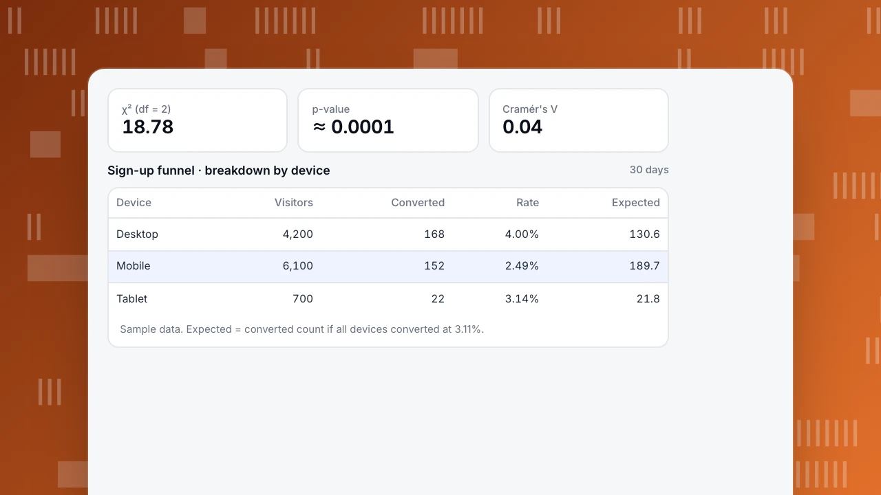
Step 4: decide. 18.78 is far above 5.99; p ≈ 0.0001. Conversion is not independent of device.
Step 5: where is the difference, and how big? The contributions show it: desktop converts more than expected, mobile less, tablet exactly as expected. The effect size, Cramér's V = √(χ² ÷ (N × (k − 1))) = √(18.78 ÷ 11,000) = 0.04, is small. With 11,000 visitors, even modest gaps are "significant". The business question is whether a 1.5-point mobile gap is worth fixing (it usually is: 6,100 mobile visitors × 1.5 points ≈ 92 conversions a month).
χ² (df = 2)
18.78
p-value
≈ 0.0001
Cramér's V
0.04
Sign-up funnel · breakdown by device
30 days| Device | Visitors | Converted | Rate | Expected |
|---|---|---|---|---|
| Desktop | 4,200 | 168 | 4.00% | 130.6 |
| Mobile | 6,100 | 152 | 2.49% | 189.7 |
| Tablet | 700 | 22 | 3.14% | 21.8 |
Sample data. Expected = converted count if all devices converted at 3.11%.
Worked example 2: sample ratio mismatch
An experiment was set up to split users 50/50. After two weeks: 50,410 in control and 49,180 in the variant (total 99,590). Expected under 50/50: 49,795 each.
χ² = (50,410 − 49,795)² ÷ 49,795 + (49,180 − 49,795)² ÷ 49,795 = 7.60 + 7.60 = 15.19, df = 1, p ≈ 0.0001.
A 50.6 / 49.4 split looks harmless, but with this many users it is very unlikely to be chance. This is a sample ratio mismatch (SRM): something in assignment or tracking is broken (a redirect losing users in one arm, bots, a script loading late). Results from an experiment with SRM should not be trusted until the cause is found. Many experimentation teams run this check automatically with a strict threshold such as p < 0.001.
Assumptions and when not to use it
- Counts, not percentages or averages. Convert rates back to counts first.
- Independent observations. Each person counted once. If one user has many sessions, count users or use a method that handles repeats.
- Expected count of at least 5 in each cell (a common rule; some texts allow up to 20% of cells between 1 and 5). Otherwise merge categories or use Fisher's exact test, which is standard for small 2×2 tables.
- Mutually exclusive categories. A visitor cannot be both mobile and desktop in the same table.
Chi-square vs other tests
| Data | Test |
|---|---|
| Counts in categories | Chi-square (or Fisher's exact for small samples) |
| Two proportions, two groups | Two-proportion z-test (same result as 2×2 chi-square without continuity correction) |
| Averages of two groups | t-test |
| Averages of three or more groups | ANOVA |
| How an outcome depends on several inputs | Regression, for example logistic regression |
| Data | Test |
|---|---|
| Counts in categories | Chi-square or Fisher exact |
| Two proportions | Two-proportion z-test |
| Two averages | t-test |
| Several averages | ANOVA |
| Several inputs | Regression |
A 2×2 chi-square without continuity correction equals the two-proportion z-test squared.
Common mistakes
- Treating "significant" as "important". Large analytics samples make tiny differences significant; report the effect size and the absolute difference.
- Testing many breakdowns and reporting the one that hits. Ten segments at α = 0.05 give a good chance of a false positive; use a correction such as Bonferroni. See also type I and type II errors.
- Counting sessions as independent people. Inflates the sample and the χ².
- Ignoring mix effects. A device gap can come from channel mix (mobile traffic is mostly social); check within channels to avoid Simpson's paradox.
- Stopping at "they differ". The test says the table is not random; the contributions and rates tell you where.
Running it on TapCub data
Build a funnel or a goal report broken down by device, channel or country, and read off the count of people who reached each step and who did not. Those counts go straight into the table above; any spreadsheet (CHISQ.TEST) or Python (scipy.stats.chi2_contingency) does the rest. TapCub does not run A/B tests itself, but if you send the variant name as an event property from your experiment tool (custom events), you can count users per variant and run the SRM check from example 2.
See also: Inferential statistics.
Sources
- NIST/SEMATECH. e-Handbook: chi-square goodness-of-fit test.
- Penn State STAT 500. Chi-square test of independence.
- Fabijan, A. et al. (2019). Diagnosing sample ratio mismatch in online controlled experiments. KDD 2019.
Was this article helpful?
We use your answers to fix and expand this page.
Couldn’t send. Please try again in a minute.
Thanks for the feedback. We’ll use it to improve this page.You’ve already sent feedback on this page. Thanks.

Product Analyst
Focuses on event analysis, conversion funnels, and retention, using clear metric definitions and structured analysis to explain product performance.