Try it on your own data
Every report in this article is in the free plan. One snippet for web and apps, up to 10 sites.
Start freeThe Bonferroni correction divides your significance level by the number of comparisons. With a control and five variants at α = 0.05, each test must reach p < 0.01. In our example, four variants look significant on their own, but only one survives the correction; Holm's method keeps two. The price of the stricter threshold is about 49% more traffic per arm. Decide the number of comparisons before you look at results.
What you will learn
- Five variants at α = 0.05 give a 22.6% chance of at least one false winner; Bonferroni sets each test to 0.01
- In the sample, 4 of 5 variants are raw winners, 1 survives Bonferroni and 2 survive Holm
- The stricter threshold needs about 49% more visitors per arm to detect the same lift
What does the Bonferroni correction do?
The Bonferroni correction keeps the chance of at least one false positive across a whole set of tests at your chosen level. You divide the significance level by the number of comparisons: adjusted α = α ÷ number of comparisons. Statsig's documentation defines it the same way, as the experiment's significance level divided by the number of comparisons, applied to test groups, to metrics, or to both (Statsig). The NIST handbook expresses the same idea for intervals: build each of g intervals at confidence level 1 − α/g, and the overall confidence is at least 1 − α (NIST).
Take α = 0.05 and 5 comparisons. Each test must now clear 0.05 ÷ 5 = 0.01. A p-value of 0.03, which looks significant on its own, no longer counts. The correction guards against false positives; it does not make a weak result stronger. The rest of this guide is one worked example, the price you pay in sample size, and a rule for when to apply it. If you want the definition first, read the Bonferroni correction glossary entry; for what significance means, see statistical significance.
Why testing five variants breaks the 5% rule
A 5% significance level means a test with no real effect still shows "significant" 1 time in 20. Run several tests and those chances add up; nothing about the individual tests is unusual, and the inflation comes purely from the number of looks. For k independent tests with no real effect, the probability of at least one false positive is 1 − (1 − α)^k:
| Number of tests (k) | Chance of at least one false positive at α = 0.05 | Bonferroni per-test α |
|---|---|---|
| 1 | 5.0% | 0.0500 |
| 3 | 14.3% | 0.0167 |
| 5 | 22.6% | 0.0100 |
| 10 | 40.1% | 0.0050 |
| 20 | 64.2% | 0.0025 |
We checked the 5-test row by simulation: in 200,000 runs of five tests where nothing was really different, 22.5% produced at least one "significant" result at 0.05, and only 4.9% did at a per-test level of 0.01. So the correction brings the family back to about the 5% you promised. A control with five variants is exactly this situation: five comparisons, one family. The same arithmetic applies to metrics, so five metrics on one variant are also five comparisons.
| Number of tests | Chance of at least one false positive | Bonferroni per-test α |
|---|---|---|
| 1 | 5.0% | 0.0500 |
| 3 | 14.3% | 0.0167 |
| 5 | 22.6% | 0.0100 |
| 10 | 40.1% | 0.0050 |
| 20 | 64.2% | 0.0025 |
Independent tests with no true effect, α = 0.05. Probability = 1 − 0.95^k.
Worked example: control and five variants
Sample data: a landing-page test with a control and five new headlines, each shown to 10,000 visitors. The control converts 500 of 10,000 (5.0%). Each variant is compared with the control using a two-sided two-proportion z-test.
| Variant | Conversions | Rate | Relative lift | Raw p-value | Significant at 0.05? | Bonferroni-adjusted p (× 5) | Significant at family 0.05? |
|---|---|---|---|---|---|---|---|
| A | 590 | 5.90% | +18.0% | 0.0051 | Yes | 0.0253 | Yes |
| B | 580 | 5.80% | +16.0% | 0.0123 | Yes | 0.0616 | No |
| C | 572 | 5.72% | +14.4% | 0.0238 | Yes | 0.1190 | No |
| D | 566 | 5.66% | +13.2% | 0.0377 | Yes | 0.1887 | No |
| E | 510 | 5.10% | +2.0% | 0.7468 | No | 1.0000 | No |
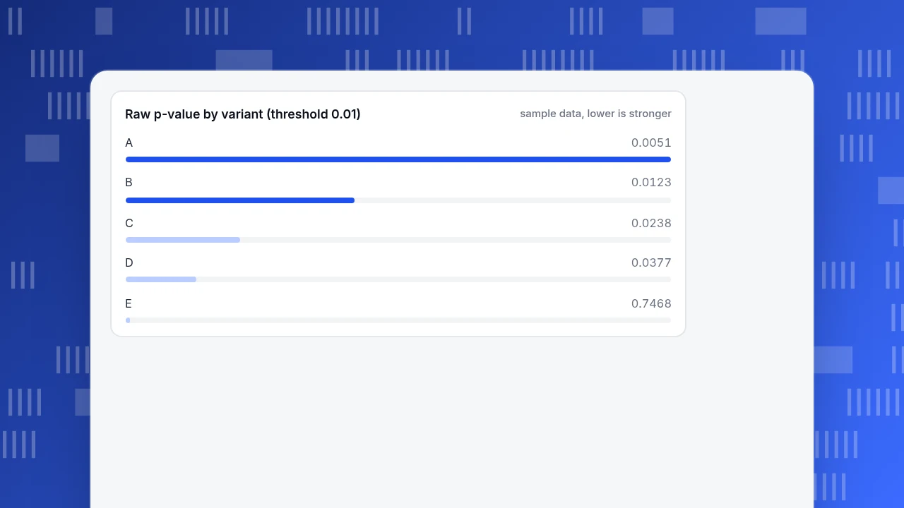
Without a correction, four of five variants look like winners. With Bonferroni, only A clears the bar: its p-value 0.0051 is below 0.01, or equivalently 5 × 0.00506 = 0.0253 is below 0.05. B, C and D have real-looking lifts, but the evidence for each is not strong enough once you admit that you looked at five variants.
Read the result carefully. "Not significant after correction" does not mean "no effect". It means you cannot rule out chance at the family level. B's lift of 16% is still the best estimate; you just cannot claim it with the same confidence.
Raw p-value by variant (threshold 0.01)
sample data, lower is strongerWhat the correction costs in sample size
A stricter threshold needs more data to detect the same lift. To detect a rise from 5.0% to 6.0% with 80% power and a two-sided test:
| Per-test α | Visitors needed per arm | Total with control and 5 variants |
|---|---|---|
| 0.05 (no correction) | 8,158 | 48,948 |
| 0.01 (Bonferroni, 5 tests) | 12,139 | 72,834 |
That is 48.8% more traffic per arm. Two honest options follow: collect the extra visitors, or test fewer variants. Budget the extra traffic before launch, because stopping a test early to save time is the quickest way to invalidate it. Dropping from five variants to two cuts the per-test α only to 0.025 and saves traffic as well as correction cost. For how sample size, power and minimum detectable effect fit together, see statistical power and the minimum detectable effect.
Holm: a correction with more power
Bonferroni is simple but conservative. The Holm step-down method gives the same guarantee on the family-wise error rate and rejects at least as many hypotheses (Holm, 1979). Sort the p-values from smallest to largest and compare the i-th smallest with α ÷ (k − i + 1), stopping at the first one that fails:
| Rank | Variant | p-value | Threshold α ÷ (5 − rank + 1) | Decision |
|---|---|---|---|---|
| 1 | A | 0.0051 | 0.0500 ÷ 5 = 0.0100 | Reject |
| 2 | B | 0.0123 | 0.0500 ÷ 4 = 0.0125 | Reject |
| 3 | C | 0.0238 | 0.0500 ÷ 3 = 0.0167 | Stop: not significant |
| 4–5 | D, E | Not tested |
Holm keeps A and B where Bonferroni keeps only A. The error guarantee is the same, so if you are correcting anyway there is little reason not to use Holm. Use plain Bonferroni when you want a single threshold to state in advance or a simple sentence for a report. Both methods can be computed in a spreadsheet.
Adjusted confidence intervals
If you report intervals, adjust them with the same logic. With 5 comparisons, a family 95% confidence level means building each interval at 1 − 0.05 ÷ 5 = 99%:
| Variant | Difference vs control (points) | Unadjusted 95% interval | Bonferroni 99% interval |
|---|---|---|---|
| A | +0.90 | +0.27 to +1.53 | +0.07 to +1.73 |
| B | +0.80 | +0.17 to +1.43 | −0.02 to +1.62 |
| C | +0.72 | +0.10 to +1.34 | −0.10 to +1.54 |
| D | +0.66 | +0.04 to +1.28 | −0.16 to +1.48 |
Report the adjusted interval next to the adjusted p-value so readers can see both. The intervals tell the same story as the p-values, with more information: A's interval stays above zero, B's just touches it, and the width shows how little the data constrain the size of the lift.
When to use it, and when not to
- Decide the family before you look. Count the comparisons you will report as findings: five variants against one control is k = 5. Counting after you see the results lets you quietly shrink k.
- Correct the headline claim, not every number. If you have one primary metric and several secondary ones, give the primary the biggest share. Statsig's documented example gives primary metrics 60% of α: with 2 primary metrics each gets 0.6 × 0.05 ÷ 2 = 0.015, and with 4 secondary metrics each gets 0.4 × 0.05 ÷ 4 = 0.005 (Statsig).
- Switch methods when k is large. With dozens of metrics or segments, Bonferroni becomes very strict. Controlling the false discovery rate is the usual alternative; see false discovery rate.
- Do not correct a single pre-planned test. One question, one test, one threshold.
- Do not split a result after the fact. Slicing a failed test by country, device and new versus returning creates new comparisons; each slice counts toward k.
Four mistakes that undo the correction
- Choosing the method after seeing the results. Trying Bonferroni, then Holm, then no correction, and keeping whichever shows a winner, adds more comparisons. Fix the method before the test.
- Counting only the variants that survived. If you launched five variants and dropped two before reporting, k is still 5, because the two you dropped were also looked at.
- Correcting the p-value but not the story. "Not significant after correction" is not "no effect". Report the estimate and the adjusted interval, as in the table above, and say what range of lifts the data still allows.
- Peeking and stopping early. Checking daily and stopping the day one variant passes inflates false positives beyond what Bonferroni covers. Set the sample size from the cost table first and read the result once it is reached.
Doing this with your own data in TapCub
Take the five-variant example above. TapCub does not run A/B tests or split traffic, so variant assignment comes from your own code or testing tool; what TapCub does well is count what each variant did.
- Send variant-specific events. Fire an exposure event and a sign-up event per variant, for example
exposure_a,signup_a,exposure_b,signup_b. You can also sendvariantas an event property, which you can read with the SQL console below. - Build one funnel per variant. In All-platform analytics › Behavior › Behavior analysis, make a funnel from
exposure_atosignup_a, and repeat for each variant. By default a funnel counts the first entry per person per session, then distinct people. - Read each variant's rate. Each step shows its count and the rate against the previous step; export the table as CSV, or use the SQL console under Metrics & SQL to group the raw event counts by the
variantproperty. - Apply the correction yourself. The funnel reports counts and rates; dividing α by the number of variants, or running Holm, is the arithmetic above, done in a spreadsheet. A bot-filtered denominator matters too: TapCub keeps crawlers out of the visitor counts that feed conversion rates.
- Mark the change. Add a date annotation under Configuration › Annotations for the day the test started and stopped, so later readers can tie the numbers to the test.
TapCub measures the outcome; it does not assign variants, calculate corrected p-values or declare winners. For the broader question of significance, see statistical significance example and how to interpret a p-value.
FAQ
What is the Bonferroni correction in simple terms?
It is a way to stay honest when you run several tests at once. You divide your significance level by the number of tests, so with α = 0.05 and 5 tests each must reach p < 0.01. That keeps the chance of any false positive across all five near 5%.
How do you calculate the Bonferroni correction?
Divide α by the number of comparisons: adjusted α = α ÷ k. Alternatively multiply each p-value by k, cap it at 1, and compare it with the original α. For five tests at 0.05, the threshold is 0.01, and a raw p of 0.00506 becomes 0.0253 after multiplying by 5.
When should you not use the Bonferroni correction?
Skip it for one pre-planned test, and consider something else when k is large. With many tests it becomes very conservative and misses real effects. Holm gives equal protection with more power, and false discovery rate control suits dozens of metrics where a few false leads are acceptable.
Is Bonferroni too conservative?
It can be. It assumes the worst case for dependence between tests, so its real error rate is often below the target and it may reject too few true effects. In the example it kept 1 of 4 raw winners where Holm kept 2. The price is extra sample size, about 49% more per arm here.
Should I correct for multiple metrics as well as multiple variants?
Yes if you will act on any of them. Treat every comparison you report as a finding as part of the family, or split α between primary and secondary metrics before the test. A common pattern is 60% of α for primary metrics and 40% for secondary, divided equally within each group.
Sources
- Statsig, Bonferroni correction (definition, per-metric tier example with α = 0.05). Checked 2026-11-20.
- NIST/SEMATECH e-Handbook of Statistical Methods, Bonferroni method (α/g intervals and overall confidence at least 1 − α). Checked 2026-11-20.
- Holm, S. (1979), A simple sequentially rejective multiple test procedure, Scandinavian Journal of Statistics 6(2), 65–70.
- Bland, J. M. and Altman, D. G. (1995), Multiple significance tests: the Bonferroni method, BMJ 310, 170 (background reading).
Was this article helpful?
We use your answers to fix and expand this page.
Couldn’t send. Please try again in a minute.
Thanks for the feedback. We’ll use it to improve this page.You’ve already sent feedback on this page. Thanks.

Data Analyst
Explores traffic sources, conversion funnels, and retention, using clear metric definitions and concrete examples to explain what the numbers mean.