Try it on your own data
Every report in this article is in the free plan. One snippet for web and apps, up to 10 sites.
Start freeA statistical significance example: a control converts 480 of 10,000 visitors (4.80%) and a variant 540 of 10,000 (5.40%). The two-proportion z-test gives z = 1.93 and p = 0.054, so the 12.5% lift is not significant at the 5% level. Below is every step of that calculation, the interval and sample size behind it, and the rule for deciding whether to ship.
What you will learn
- Fix the hypotheses, the 0.05 level and the sample size before looking: z = 1.93 and p = 0.054 is a miss, not a near win
- Report the confidence interval (-0.01 to +1.21 points) and power (about 49%), not only the verdict
- Stopping when the number turns significant can push the real false-positive rate far above 5%
What is the test, and what do we decide before looking at data?
A statistical significance test answers one question: if the two versions really converted equally well, how surprising would the gap we saw be? Here is a concrete case. A checkout page has a control (A) and a variant (B) with a shorter form. Each version was shown to 10,000 visitors, assigned at random by your testing tool.
Sample data:
| Visitors | Orders | Conversion rate | |
|---|---|---|---|
| Control (A) | 10,000 | 480 | 4.80% |
| Variant (B) | 10,000 | 540 | 5.40% |
B looks better: 0.60 percentage points higher, a relative lift of 12.5%. Whether that is real or luck is what the test decides.
Write down three things before you look, because choosing them after the result lets the result steer them:
- Hypotheses. The null hypothesis says the true conversion rates are equal (pA = pB). The alternative says they differ (two-sided).
- Significance level. We use α = 0.05: we accept a 5% chance of calling a difference real when there is none.
- Sample size and stopping rule. Decide how many visitors each version gets and do not stop early. The section on sample size below shows why. A one-line plan is enough: two-sided test, α = 0.05, 21,103 visitors per version, one look.
The same logic applies to any two-group comparison; the full explanation of the idea is in statistical significance, and the quantity we compute is the p-value.
How do you calculate it, step by step?
For two conversion rates the standard method is the two-proportion z-test, described in the NIST/SEMATECH e-Handbook. It works when each group has enough conversions and non-conversions (a common rule is at least 10 of each; here we have 480 and 9,520, so it is fine).
| Step | Formula | Calculation | Result | ||
|---|---|---|---|---|---|
| 1. Rates | p̂ = orders ÷ visitors | A: 480 ÷ 10,000; B: 540 ÷ 10,000 | 0.0480 and 0.0540 | ||
| 2. Pooled rate | p̂ = (x₁ + x₂) ÷ (n₁ + n₂) | (480 + 540) ÷ 20,000 | 0.0510 | ||
| 3. Standard error | √( p̂(1 − p̂)(1/n₁ + 1/n₂) ) | √(0.051 × 0.949 × 0.0002) | 0.003111 | ||
| 4. z statistic | (p̂B − p̂A) ÷ SE | 0.0060 ÷ 0.003111 | 1.93 | ||
| 5. p-value | 2 × (1 − Φ(\ | z\ | )) | 2 × (1 − Φ(1.93)) | 0.054 |
Why pool the rates in step 2? The null hypothesis says both groups share one true rate, so the best single estimate of it uses all 20,000 visitors. The decision rule from the handbook for a two-sided test: reject the null hypothesis if |z| is greater than 1.96, which is the value that leaves 2.5% in each tail at α = 0.05.
Our |z| is 1.93, just under 1.96, and the p-value is 0.054, just over 0.05. The result is not statistically significant at the 5% level.
| Result | What it says | What to do |
|---|---|---|
| p < 0.05, whole interval above break-even | Likely real and worth having | Ship |
| p < 0.05, interval reaches below break-even | Likely real, may be too small | Ship only if cheap and reversible |
| p >= 0.05, wide interval | Inconclusive, often underpowered | Run to the planned sample, or test a bigger change |
| p >= 0.05, narrow interval around 0 | Probably no effect worth having | Stop and try something else |
Break-even lift is the smallest lift that repays the cost of the change; compute it before the test.
What does "not significant" mean here, and what does it not mean?
It does not mean there is no difference. It means the data are not surprising enough, under "no difference", to reject it with the evidence we set out to require. The American Statistical Association's 2016 statement on p-values puts the limits plainly: a p-value does not measure the probability that the hypothesis is true, and it does not measure the size or importance of an effect.
A confidence interval says more than the yes/no verdict. For the difference in rates, use the unpooled standard error, √(0.048 × 0.952 ÷ 10,000 + 0.054 × 0.946 ÷ 10,000) = 0.003111 (the same to four digits here). The 95% interval is 0.0060 ± 1.96 × 0.003111, which is −0.01 to +1.21 percentage points.
Report the two numbers together: the p-value says how surprising the gap is, and the interval says how large it might be. Read it like this:
- The interval just barely includes zero, which is why p is just above 0.05. The two always agree.
- The plausible lifts run from roughly nothing to 1.21 points, more than double the observed 0.60.
- A non-significant result is still a result: record it, so the idea is not retried blindly later.
- So the honest summary is not "B did not win" but "B may help by up to about a point, and we have not collected enough data to tell".
The study is also underpowered. If the true lifts really are 4.80% versus 5.40%, a test with 10,000 visitors per version detects it only about 49% of the time at α = 0.05. A coin-flip chance of success is not a design anyone would choose on purpose. Power is the chance that a test detects an effect that is really there, and 80% is the usual target; the next section shows the sample that reaches it.
What happens if you keep collecting data until it is significant?
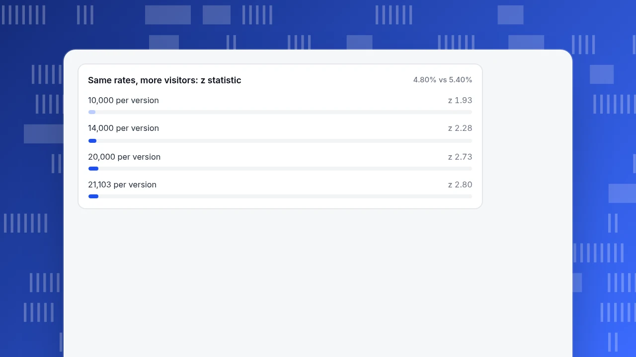
The tempting move is to wait a few more days. Here is what the same rates would show at larger samples, assuming 4.80% and 5.40% hold exactly:
| Visitors per version | Orders A / B | z | Two-sided p | Significant at 0.05? |
|---|---|---|---|---|
| 10,000 | 480 / 540 | 1.93 | 0.054 | No |
| 14,000 | 672 / 756 | 2.28 | 0.022 | Yes |
| 20,000 | 960 / 1,080 | 2.73 | 0.006 | Yes |
| 21,103 | 1,013 / 1,140 | 2.80 | 0.005 | Yes |
The table shows that more data would resolve the question if the rates held. It does not show that you may stop at 14,000. Evan Miller's analysis of repeated testing shows what goes wrong: if you check after every observation and stop the first time you see 5% significance, the real false-positive rate can reach 26.1% in the example he gives (a 50% baseline, stopping by 150 observations), more than five times the intended level. Even 10 looks at a 1% threshold behave like roughly 5%.
A fixed-sample test is read once; that is the price of its 5% guarantee. The rules that keep a test honest:
- Fix the sample size before the test starts, and read the result once, when you reach it. A common way to size it for 80% power at α = 0.05 is n ≈ 16 × p(1 − p) ÷ d² per group, where d is the smallest difference you care about. For p = 4.8% and d = 0.6 points, that gives 16 × 0.048 × 0.952 ÷ 0.006² ≈ 20,300 per version. The full formula, which accounts for both rates, gives 21,103 per version.
- If you must check early, use a method built for it (sequential testing, or a stricter threshold for interim looks) rather than the standard test read repeatedly.
- Never extend a test only because the first answer was not the one you wanted.
Same rates, more visitors: z statistic
4.80% vs 5.40%Is a significant result worth acting on?
Significance says the gap is probably not luck. It does not say the gap is worth the effort. Add the arithmetic that your finance team will, starting with the break-even lift: the cost of the change ÷ margin per order ÷ monthly visitors. Here 6,000 ÷ 24 ÷ 100,000 = 0.25 percentage points, the smallest lift that repays the change within one month.
| Quantity | Sample value |
|---|---|
| Visitors per month to the checkout page | 100,000 |
| Observed lift | +0.60 points = 600 extra orders per month |
| Margin per order | $24 |
| Extra margin | 600 × $24 = $14,400 per month |
| Cost of the change (design, development, testing) | $6,000 |
| Payback at the observed lift | 6,000 ÷ 14,400 ≈ 0.4 months |
| Payback at the lower end of the interval (≈ 0 extra orders) | Never; the change has no benefit |
The last row is the reason to look at the interval: the decision to ship can be made on the observed lift, but the risk is the lower bound.
Before committing budget, rerun the payback using the interval's lower end. A simple decision rule for any test:
- p < 0.05 and the whole interval is above your break-even lift: ship.
- p < 0.05 but the interval's lower end is below break-even: ship only if the change is cheap and easy to reverse.
- p ≥ 0.05 and the interval is wide: inconclusive. Run longer to the planned sample size, or test a bigger change.
- p ≥ 0.05 and the interval is narrow around zero: there is probably no effect worth having. Stop and try something else.
How do you measure the two groups in TapCub?
Take the checkout example above. TapCub does not split traffic or compute a p-value; your testing tool or your own code assigns visitors to A or B. TapCub's job is to count what each group did, with bots kept out of the visitor base. The steps:
- Send the variant with the event. When a visitor completes checkout, call
tapcub.track('order_complete', { variant: 'B' })from your code, and send the variant on the earlier event too, so the same property exists at every funnel step. - Build the funnel. In All-platform analytics › Behavior › Behavior analysis, make a funnel from the checkout-start event to
order_complete, and break it down byvariant. Each step shows counts and the rate against step one; the default counting is unique, so each visitor is counted once. - Check the denominators first. Both groups should be close to the planned 10,000. If one is far off, the split is broken, and the result means nothing until it is fixed.
- Copy the counts into the formula. The visitors and orders per group are the x and n of the table above. Do the arithmetic in a spreadsheet or script.
- Keep bots out. TapCub counts recognized bots and AI crawlers separately in Web analytics › Bots, so they do not enter the visitor and conversion counts you copy.
For site-wide goals rather than one funnel, Web analytics › Goals shows conversions, converting visitors and the overall conversion rate for the selected dates.
What mistakes ruin a significance test?
- Stopping when the number looks good. Covered above; it inflates false positives.
- Running many comparisons and reporting the winner. Testing 20 variants at α = 0.05 gives a high chance that one looks significant by luck. Divide α by the number of comparisons, or fix the one comparison you care about in advance.
- Using the test on unequal or overlapping groups. If the same visitor sees both versions, or the groups were not randomly assigned, the standard error is wrong.
- Treating p = 0.054 and p = 0.046 as opposites. They are almost the same evidence. Report the interval, not only the verdict.
- Slicing the result after the fact. Splitting a finished test by device, country or channel and reporting the one slice that is significant is the same multiple-comparison problem. Decide the segments you will look at before the test starts.
- Confusing significance with size. A very large sample makes tiny differences significant; always check the interval against the break-even lift.
FAQ
What is an example of statistical significance?
A checkout test with 10,000 visitors per version, 480 orders for the control and 540 for the variant. The two-proportion z-test gives z = 1.93 and p = 0.054. At α = 0.05 that is not significant. With 20,000 visitors per version and the same rates, z = 2.73 and p = 0.006, which would be.
How do you calculate statistical significance for two conversion rates?
Compute each rate, pool them into one rate using all visitors, then divide the difference by the standard error √(p̂(1 − p̂)(1/n₁ + 1/n₂)) to get z. Convert z to a two-sided p-value and compare it with your α, usually 0.05. The formula is in the NIST/SEMATECH handbook.
What p-value is statistically significant?
By convention, a p-value below the significance level you chose before the test, most often 0.05. The level is a choice about how much false-positive risk you accept, not a law of nature. The American Statistical Association warns against treating 0.05 as a bright line that decides truth. Report the exact p-value and the interval, not just "p < 0.05".
Does a non-significant result mean there is no difference?
No. It means the data are not strong enough to rule out chance at your chosen level. Look at the confidence interval: in this example it runs from −0.01 to +1.21 points, so a real lift of about a point is still plausible. The test was underpowered.
How many visitors do I need for an A/B test?
It depends on the baseline rate and the smallest lift you care about. For a 4.8% baseline and a 0.6-point lift, at 80% power and α = 0.05, you need about 21,100 visitors per version. A rough check is n ≈ 16 × p(1 − p) ÷ d² per group. Smaller expected lifts need far more visitors: halving d roughly quadruples n.
Sources
- NIST/SEMATECH e-Handbook of Statistical Methods, Do two processes produce the same proportion of defectives? (pooled two-proportion z-test and critical-value rule). Checked 2026-11-20.
- Ronald L. Wasserstein & Nicole A. Lazar, The ASA's Statement on p-Values: Context, Process, and Purpose, The American Statistician 70(2), 129–133, 2016.
- Evan Miller, How Not To Run An A/B Test (26.1% false-positive rate under continuous peeking; stopping at 150 observations, 50% baseline). Checked 2026-11-20.
Was this article helpful?
We use your answers to fix and expand this page.
Couldn’t send. Please try again in a minute.
Thanks for the feedback. We’ll use it to improve this page.You’ve already sent feedback on this page. Thanks.

Product Experience Specialist
Writes about product experience, practical workflows, and growth, turning complex processes into clear steps for everyday decisions.