Try it on your own data
Every report in this article is in the free plan. One snippet for web and apps, up to 10 sites.
Start freeA confounding variable is a third factor that differs between the groups you compare and also affects the outcome, so it makes a gap look like cause and effect. The fix is one move: split the result by the suspect (channel, device, new or returning, plan) and check whether the gap survives inside each slice. Below are three recomputable examples and the methods that follow.
What you will learn
- Split any gap by the usual suspects before believing it: channel, device, new vs returning, plan, country, signup date
- A confounder can shrink, erase or even reverse an effect, so compare the mix of each group, not only the rates
- Only randomising covers confounders you did not measure; otherwise say what you adjusted for, not that you proved a cause
What has to be true for a variable to confound?
A variable confounds a comparison when three things hold at once:
- It differs between the groups you compare. Feature users are mostly on the paid plan; non-users are mostly on the free plan.
- It affects the outcome on its own. Paid users retain better whether or not they touch the feature.
- It is not a step between the cause and the effect. Plan was chosen before the feature was used; it is not something the feature produced.
When all three hold, part of the gap you see belongs to the third variable, and the comparison credits it to the thing you were looking at. Statisticians call this a failure of exchangeability: the two groups would have behaved differently even if the feature had not existed. The formal treatment is in Greenland, Robins and Pearl (1999); the plain-language definition is already covered in confounding variable, so this guide spends its time on examples you can recompute.
The practical test is short: take the gap, split it by the suspect variable, and see whether it survives inside each slice. Everything below is that one move, repeated.
Example 1: people who use a feature retain better
Sample data: 10,000 new users, 2,000 of whom used a new "saved views" feature in their first week. Day-30 retention looks like this:
| Group | Users | Retained at day 30 | Retention |
|---|---|---|---|
| Used the feature | 2,000 | 1,040 | 52% |
| Did not use it | 8,000 | 1,920 | 24% |
The gap is 28 points, and the natural reading is that the feature doubles retention. Now split by plan, the obvious suspect, since paying customers are both more likely to explore features and more likely to stay:
| Plan | Group | Users | Retained | Retention |
|---|---|---|---|---|
| Paid | Used the feature | 1,600 | 960 | 60% |
| Paid | Did not use it | 800 | 480 | 60% |
| Free | Used the feature | 400 | 80 | 20% |
| Free | Did not use it | 7,200 | 1,440 | 20% |
Inside each plan the gap is zero. Retention is 60% for paid users and 20% for free users, with or without the feature. The 28-point gap came entirely from the mix: 80% of feature users are paid, against 10% of non-users (800 of 8,000). The mix is exactly what the checklist above describes: the variable differs between the groups, it drives the outcome, and it came first.
That is the extreme case, chosen so the arithmetic is easy to follow. Real data rarely collapses to zero; more often the gap shrinks to a fraction of its raw size. The habit that matters is the same: never report the raw gap until you have seen the sliced one.
Example 2: visitors from email convert better
Sample data: 20,000 sessions in a month, 2,000 of them from an email campaign. The raw numbers:
| Source | Sessions | Orders | Conversion rate |
|---|---|---|---|
| 2,000 | 154 | 7.7% | |
| Everything else | 18,000 | 540 | 3.0% |
Email converts at 2.57 times the rate of everything else. Before moving budget, split by new versus returning visitors. Email lists contain people who already bought, so they are mostly returning visitors.
| Visitor type | Source | Sessions | Orders | Rate |
|---|---|---|---|---|
| Returning | 1,600 | 144 | 9.0% | |
| Returning | Everything else | 3,000 | 240 | 8.0% |
| New | 400 | 10 | 2.5% | |
| New | Everything else | 15,000 | 300 | 2.0% |
Email still wins in both slices, but the lead is 1 point among returning visitors and half a point among new ones, nowhere near 4.7 points. To put one number on it, ask what the non-email group would have converted at if it had email's visitor mix (80% returning, 20% new): 0.8 × 8.0% + 0.2 × 2.0% = 6.8%. Against that baseline, email's 7.7% is a lift of 0.9 points, not 4.7. This is called direct standardisation, and it is the cheapest way to compare groups with different compositions.
The campaign did not do nothing. It did about a fifth of what the raw comparison suggested, and the rest was the audience it was sent to.
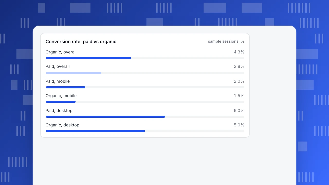
Example 3: paid traffic converts worse, until you split by device
Sample data: 10,000 paid sessions and 10,000 organic sessions.
| Channel | Overall rate | Mobile | Desktop |
|---|---|---|---|
| Paid | 2.8% (280 of 10,000) | 2.0% (160 of 8,000) | 6.0% (120 of 2,000) |
| Organic | 4.3% (430 of 10,000) | 1.5% (30 of 2,000) | 5.0% (400 of 8,000) |
Overall, organic beats paid by 1.5 points. On mobile, paid beats organic (2.0% against 1.5%). On desktop, paid beats organic (6.0% against 5.0%). The channel that looks worse is better in every slice, because 80% of paid sessions are on mobile, which converts at a third of desktop's rate or less in both channels. This reversal is Simpson's paradox, and it is the most dramatic form of confounding; the pattern is explained further in Simpson's paradox. Bickel, Hammel and O'Connell (1975) analysed a real case in university admissions, where an apparent bias in the combined figures largely disappeared once applications were compared department by department.
If you had cut the paid budget on the strength of the overall numbers, you would have cut the channel that performs better on both devices. The right comparison is by device, or standardised to a common mix: at 50/50 mobile and desktop, paid is 4.0% and organic 3.25%.
Conversion rate, paid vs organic
sample sessions, %How do you spot a confounder before it misleads you?
Three checks, in the order they pay off:
- Ask who ends up in each group. Any comparison between people who chose something (used a feature, opened an email, clicked an ad) has a selection step. If people sorted themselves, assume they differ on something else too. See selection bias.
- Split by the usual suspects. In product and marketing data the list is short: acquisition channel, device, new versus returning, plan or customer size, country, and signup date (seasonality and releases). If the gap survives each split, it is far more believable.
- Compare the mix, not just the rates. If the shares of mobile, returning or paid users differ a lot between the groups, you have found the candidate. In Example 1 the mix was 80% against 10%.
A gap that changes a lot when you split, shrinks, vanishes or flips, is confounded. A gap that holds roughly steady in every slice is not proof of cause, but you have removed the most common explanation.
What can you do about it?
| Method | What it does | Works when | Weak spot |
|---|---|---|---|
| Stratify | Compare inside slices (plan, device) and report each | Few confounders, enough users per slice | Slices get thin fast |
| Standardise | Reweight to one common mix and compare rates | You want a single comparable number | Hides differences between slices |
| Match | Pair each treated user with a similar untreated one | Many confounders you have measured | Only handles what you measured |
| Randomise | Assign the treatment by chance | You control the treatment | Needs the ability to run an experiment |
Randomisation is the only method that also handles confounders you did not think of or cannot measure, which is why it is the standard for causal claims. Propensity-score methods (Rosenbaum and Rubin, 1983) are a formal way to do matching, but they too can only adjust for variables that are recorded. If you cannot run an experiment, the honest wording is "after accounting for plan and device, feature users retained X points better", not "the feature raised retention by X points". For the wider causal question see correlation vs causation.
| Method | What it does | Weak spot |
|---|---|---|
| Stratify | Compare inside slices such as plan or device | Slices get thin fast |
| Standardise | Reweight groups to one common mix | Hides differences between slices |
| Match | Pair similar treated and untreated users | Only handles measured variables |
| Randomise | Assign the treatment by chance | Needs the ability to run an experiment |
Randomisation is the only method that also covers variables you did not measure.
Which mistakes make confounding worse?
- Controlling for something the treatment causes. If the feature leads people to log in more, and you adjust for login frequency, you remove part of the real effect. Only adjust for variables that were fixed before the treatment (plan at signup, channel, device, country).
- Slicing until nothing is left. Splitting by plan, device, country and week gives cells with five users each. Rates from tiny cells swing wildly. Start with one or two splits and check the counts.
- Treating "I adjusted for it" as "I removed it". You removed the part you measured. Say what you did not measure.
- Assuming a confounder always shrinks the effect. It can hide a real effect or reverse its sign, as in Example 3.
- Looking only for the hidden variable. The confounder is often in plain sight in your own table (device, channel); it only needs a split.
How do you do these splits in TapCub?
The examples above are the three questions teams most often ask of an analytics tool. Here is how the device example runs in TapCub, using only breakdown and segment features that exist today.
- Start with the raw comparison. In All-platform analytics › Behavior › Behavior analysis, build a funnel from landing to order and look at it by channel. Funnel breakdown uses one layer and keeps the 10 groups with the most entries, so make that layer the channel.
- Add the suspect variable. In All-platform analytics › Behavior › Event analysis, count the order event with a breakdown of up to three layers, such as channel then device then new or returning visitor. Compare the conversion rate by channel inside each device, as in the table above.
- Retention needs a different route. Retention analysis has no breakdown, so build one segment per slice in All-platform analytics › Users › Segments & tags (for example "mobile") and apply each in turn, or use a filter. Anonymous visitors never join segments, so this works for identified users only.
- Ask what moved. When a number changed between two periods, the AI assistant's "why did it change" view in All-platform analytics › Operations › AI Assistant splits channel, referrer domain, country, device and entry page, and shows each value's change divided by the total change. It shows which dimension carried the movement; it does not say whether anything caused it.
- Testing the cause is outside TapCub. TapCub does not run experiments or split traffic; it only measures. Run the randomised test in your own tooling, and bring the results back as events to read by segment.
FAQ
What is an example of a confounding variable?
Plan type in a feature-retention comparison. Paid users both use more features and stay longer for other reasons, so comparing feature users with non-users mixes the feature's effect with the plan's. In the sample above, a 28-point retention gap fell to zero inside each plan.
What are confounding variables in simple terms?
A confounding variable is a third factor that is linked to both the thing you think is causing a result and the result itself, so it creates or hides a link between them. Check for one by splitting the data by that factor.
How is a confounding variable different from a lurking variable?
Many sources use the terms interchangeably. A lurking variable is usually one nobody measured; a confounder is any variable that distorts the comparison, measured or not. The fix differs: measured confounders can be adjusted for, unmeasured ones need randomisation.
Can a confounder make a real effect disappear?
Yes. A confounder can inflate an effect, hide it or reverse its direction. In the paid-versus-organic example, device mix pushed paid to the bottom overall even though it won on both devices.
How do you control for confounding variables?
Stratify (compare inside slices), standardise (reweight to a common mix), match similar users, or randomise assignment. Randomisation is the only one that also covers variables you did not measure.
See also: Confounding vs Lurking Variable: The Difference, With Worked Examples.
Sources
- Greenland, S., Robins, J. M., Pearl, J. (1999). Confounding and Collapsibility in Causal Inference. Statistical Science, 14(1), 29–46.
- Bickel, P. J., Hammel, E. A., O'Connell, J. W. (1975). Sex Bias in Graduate Admissions: Data from Berkeley. Science, 187(4175), 398–404.
- Rosenbaum, P. R., Rubin, D. B. (1983). The central role of the propensity score in observational studies for causal effects. Biometrika, 70(1), 41–55.
Was this article helpful?
We use your answers to fix and expand this page.
Couldn’t send. Please try again in a minute.
Thanks for the feedback. We’ll use it to improve this page.You’ve already sent feedback on this page. Thanks.

Technical Engineer
Focuses on tracking code, SDKs, and API integrations, with practical guidance on implementation checks and troubleshooting.