Try it on your own data
Every report in this article is in the free plan. One snippet for web and apps, up to 10 sites.
Start freeA confounding variable and a lurking variable are both a third factor linked to the cause and the effect; the usual difference is that a confounder is measured and a lurking variable is not, so only the confounder can be adjusted for. Two sample tables and the 1973 Berkeley admissions counts show why the difference matters: in the tables below, a 10.6-point deficit becomes a 3.5-point lead once you hold the confounder constant.
What you will learn
- Same problem, different visibility: a confounder is in your data and can be stratified; a lurking variable is not, until you start recording it (some sources treat the terms as synonyms)
- Pooled numbers can reverse: viewers 15.0% vs non-viewers 25.6% became +2.0 and +5.0 points within visitor type, and Berkeley's 14.1-point gap became 4.3 points in women's favour by department
- Fix by measurement: stratify and standardize what you measured, start recording what you did not, and randomize when you cannot
What is the difference between a confounding and a lurking variable?
Both are a third variable that is associated with the explanatory variable and with the response, and so can fake, hide or distort the link between them. The usual dividing line is awareness: a confounding variable is one the study has identified or measured, and a lurking variable is a confounder nobody measured, so it cannot be adjusted for. Peter Dunn's open textbook Scientific Research and Methodology puts it this way: a confounding variable is "an extraneous variable associated with the response and explanatory variables", and "some confounding variables are also called lurking variables: if they are not measured, assessed, described or recorded."
Usage varies. Some courses and sites treat the two terms as synonyms, and a few reserve "lurking" for a variable that was never even considered. If you are writing for a class or a reviewer, check which definition they use. For analytics work the measured-versus-unmeasured split is the one that changes what you do next, so this article uses it.
How do the two compare side by side?
| Confounding variable | Lurking variable | |
|---|---|---|
| Associated with both cause and effect | Yes | Yes |
| Measured in your data | Yes (or at least identified) | No |
| Can you stratify or adjust for it | Yes | Not until you measure it |
| Typical analytics example | Visitor type (new vs returning) is in your data, and mixes with who sees a feature | Customer plan size or intent is not recorded, and drives both feature use and retention |
| What it does to the result | Reverses or inflates the headline number | Same, but you cannot see why |
| First fix | Split by it, then compare within groups | Start recording it, or randomize who gets the treatment |
The table shows why the distinction matters in practice. The problem is identical in both columns; the difference is whether you can see the group split.
| Question | Confounding variable | Lurking variable |
|---|---|---|
| Linked to both cause and effect? | Yes | Yes |
| Measured in your data? | Yes, or at least identified | No |
| Can you adjust for it? | Yes: stratify, standardize, model | Not until measured |
| Typical fix | Compare within groups | Start recording it, or randomize |
Usage varies between textbooks; some treat the two terms as synonyms. This page uses measured vs unmeasured.
What does a confounder look like in a marketing report?
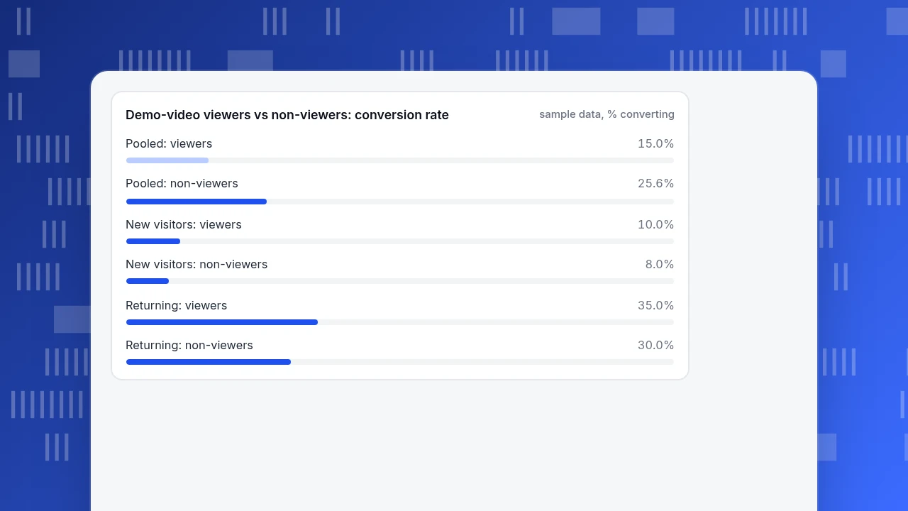
Sample data: 2,000 visitors, split by whether they watched the demo video on the pricing page, and by whether they were new or returning. The question is whether watching the video helps people buy.
| Visitor type | Watched the video | Visitors | Purchases | Rate |
|---|---|---|---|---|
| New | Yes | 800 | 80 | 10.0% |
| New | No | 200 | 16 | 8.0% |
| Returning | Yes | 200 | 70 | 35.0% |
| Returning | No | 800 | 240 | 30.0% |
Pooled, viewers bought 150 of 1,000 (15.0%), and non-viewers 256 of 1,000 (25.6%). Watching the video looks like it costs 10.6 percentage points. But within each visitor type, viewers convert better: +2.0 points among new visitors, +5.0 among returning. The pooled result reverses because viewers are mostly new visitors (800 of 1,000), who convert at a low rate whatever they watch, while non-viewers are mostly returning visitors (800 of 1,000), who are already likely to buy. Visitor type is associated with both the video and the purchase: a confounder, and since it is in the data it can be handled.
Give both groups the same visitor mix (1,000 new and 1,000 returning) and the comparison becomes: viewers 22.5%, non-viewers 19.0%, a gap of +3.5 points. This reversal pattern has a name, Simpson's paradox.
Demo-video viewers vs non-viewers: conversion rate
sample data, % convertingWhat does a lurking variable look like in a product report?
Sample data: 1,200 users, split by whether they used a reporting feature in their first month, with 90-day retention as the outcome. Account plan is not recorded in the report that someone is reading.
| Group | Users | Retained at 90 days | Rate |
|---|---|---|---|
| Used the feature | 600 | 380 | 63.3% |
| Did not use it | 600 | 216 | 36.0% |
A 27.3-point gap looks like a reason to push the feature in onboarding. Now suppose someone adds the plan as a column.
| Plan | Used the feature | Users | Retained | Rate |
|---|---|---|---|---|
| Pro | Yes | 500 | 350 | 70.0% |
| Pro | No | 100 | 66 | 66.0% |
| Free | Yes | 100 | 30 | 30.0% |
| Free | No | 500 | 150 | 30.0% |
Within Pro the gap is 4 points; within Free it is 0. Pro users are far more likely to use the feature (500 of 600) and far more likely to stay, whatever they use. With both groups standardized to the same plan mix (50% Pro), retention is 50.0% versus 48.0%, a gap of 2.0 points instead of 27.3. While the plan was not recorded, it was a lurking variable: the 27.3-point gap had a hidden driver nobody could see. Once it becomes a column, it is a confounder.
Does this happen with real data?
Yes, and the best-known case is the 1973 University of California, Berkeley graduate admissions data analysed by Bickel, Hammel and O'Connell in Science (1975). In the fall 1973 data, 8,442 men and 4,321 women applied, and about 44% of the men and 35% of the women were admitted, a gap that looked like bias against women. The authors found it came from which departments applicants chose: women applied disproportionately to departments that were harder to get into for everyone.
R's built-in UCBAdmissions dataset holds the six largest departments (4,526 applicants), which recompute like this:
| Department | Men applied | Men admitted | Women applied | Women admitted |
|---|---|---|---|---|
| A | 825 | 62.1% | 108 | 82.4% |
| B | 560 | 63.0% | 25 | 68.0% |
| C | 325 | 36.9% | 593 | 34.1% |
| D | 417 | 33.1% | 375 | 34.9% |
| E | 191 | 27.7% | 393 | 23.9% |
| F | 373 | 5.9% | 341 | 7.0% |
Pooled across the six, men were admitted at 44.5% (1,198 of 2,691) and women at 30.4% (557 of 1,835), a 14.1-point gap. Four of the six departments favour women. About 51% of the men applied to the two easiest departments (A and B), against about 7% of the women. Standardized to the same department mix, the rates are 38.7% for men and 43.0% for women. Department choice was the confounder, and it was in the data. Had admissions records not included department, it would have been a lurking variable and the headline gap would have been uninterpretable.
How do you find a confounder or lurking variable?
Ask three questions of any headline comparison, in this order.
- Who ended up in each group, and why? If people chose the treatment (watched the video, enabled the feature, started a chat), the groups differ before the treatment does. Write down the likely reasons: intent, size, tenure, device, traffic source.
- Could that reason also move the outcome? If yes, it is a candidate. Intent moves purchases; plan moves retention; department moves admission.
- Is it in the data? If yes, it is a confounder; split by it. If no, it is lurking; name it anyway, because naming it tells you what to start recording.
A quick test: split the comparison by each candidate and see whether the gap changes sign or shrinks sharply. If it does, the pooled number was telling you about the mix, not the treatment.
What do you do once you suspect one?
Which fix applies depends on what you know.
- It is measured: stratify (compare within each group, as in the tables above), then combine with standardization to a common mix. Regression with the variable as a covariate does the same job for many variables at once.
- It is unmeasured but nameable: start recording it, then re-run. For past data you may be able to reconstruct it from an existing field (plan from billing, tenure from first-seen date).
- It cannot be recorded or is unknown: randomize. Random assignment spreads every confounder, measured or not, evenly across groups on average, which is why controlled experiments are the standard route to cause. Two more rules apply to a real test: decide the sample size in advance, and do not stop early because the number looks good.
A caution on over-adjusting: do not split by a variable that is itself a consequence of the treatment (for example, "users who saw the second page" when the video is what drives people to it). That can create bias instead of removing it. The related cause-versus-pattern question is in correlation vs causation.
How do you check for confounding in TapCub?
The same check works on any dimension TapCub records. Suppose a campaign link drives one traffic source and the question is whether that source "converts worse" than another. TapCub gives you the groups and the breakdowns; it does not run experiments or assign who sees what, so fixing an unmeasured factor happens in your testing tool, not here.
- Define the purchase as a goal under All-platform analytics › Business › Goals (the same data as Web analytics › Goals). The conversion rate divides by unique visitors in the selected dates. Select the goal's row to see its source, entry page, country and device breakdowns.
- Read the pooled rate for each source first, and write it down. This is the headline number someone will quote.
- In All-platform analytics › Behavior › Behavior analysis, break the same measurement down by source and then by device (a breakdown can use up to three layers) and compare the sources inside each device. If the gap changes sign or shrinks sharply, the device mix was the confounder.
- For something TapCub does not record yet, such as the account plan, send it as an event property, or identify signed-in users with
tapcub.login, so the next report can split by it. Anonymous visitors have no user profile, so analyses built on user attributes cannot include them. - Write down what you concluded and treat any before-and-after comparison as observational: TapCub reports what happened, it does not randomize.
FAQ
What is the difference between a confounding variable and a lurking variable?
Both are third variables linked to the cause and the effect. In the common textbook usage, a confounding variable has been identified or measured, while a lurking variable is a confounder that was not measured, so it cannot be adjusted for. Some sources treat the two as synonyms.
Is a lurking variable the same as a confounder?
Not always. Many texts call a lurking variable an unmeasured confounder; others use the terms interchangeably. The practical difference is whether you can split the data by it. If you can, it is a confounder you handle; if not, it is lurking until you start recording it.
What is an example of a confounding variable?
Visitor type in the demo-video sample: new visitors mostly watched the video and mostly did not buy, returning visitors rarely watched and often bought, so the pooled result (15.0% vs 25.6%) reversed within each visitor type (+2.0 and +5.0 points).
What is an example of a lurking variable?
Account plan, in the feature-retention sample, before anyone recorded it: Pro users both used the feature more and stayed longer, so a 27.3-point retention gap shrank to 2.0 points once plan was held constant.
Can you remove a confounding variable?
You cannot remove it from reality, but you can neutralize it: stratify and standardize if it is measured, add it as a covariate in a model, or randomize assignment so it is balanced on average. Matching similar units across groups is a fourth option.
How is Simpson's paradox related?
Simpson's paradox is the extreme case: a confounder is strong enough to reverse the sign of a pooled comparison. The Berkeley and demo-video examples above both show it. If the pooled and within-group comparisons disagree, trust the within-group view only if you are sure the grouping variable is not itself an effect of the treatment.
Sources
- Dunn PK. Scientific Research and Methodology, section 6.3: Extraneous variables and variation in the response (2021) — definitions of confounding and lurking variables. Verified 2026-11-20.
- Bickel PJ, Hammel EA, O'Connell JW. Sex Bias in Graduate Admissions: Data from Berkeley. Science, 187(4175), 1975 — fall 1973 aggregate admissions and department analysis. Verified 2026-11-20.
- R Core Team. UCBAdmissions dataset documentation — the six largest departments, 4,526 applicants; totals of 2,691 men (44.5% admitted) and 1,835 women (30.4%). Verified 2026-11-20.
Was this article helpful?
We use your answers to fix and expand this page.
Couldn’t send. Please try again in a minute.
Thanks for the feedback. We’ll use it to improve this page.You’ve already sent feedback on this page. Thanks.

Customer Experience Consultant
Writes about live chat, visitor conversations, and self-service, sharing practical ways to make customer communication clearer and more effective.