Try it on your own data
Every report in this article is in the free plan. One snippet for web and apps, up to 10 sites.
Start freeEvery analytics chart is a time series, and most misreadings come from mixing up trend, weekly patterns and noise. This guide walks through four weeks of daily sessions step by step: smoothing out the weekly cycle to see the trend, measuring the weekday pattern, and catching a one-day tracking outage that a week-over-week total hid. It then covers the core techniques, forecasting baselines and common mistakes.
What you will learn
- Separate trend, seasonality and noise before judging a change
- Compare the same weekday or season, not adjacent periods
- A 7-day moving average reveals trend in daily web data
- Weekly totals can hide a one-day 20% drop
- Beat the seasonal naive forecast before trusting a model
What is time series analysis?
Time series analysis is the set of methods for studying data recorded at regular intervals, such as daily sessions, weekly sign-ups or monthly revenue, to understand how it moves over time: its long-term direction, its repeating patterns, the noise around them, and the unusual points that break the pattern. The same methods are used to forecast what comes next.
Almost every analytics chart is a time series. The difference between glancing at a line and analyzing it is separating those components, so you can tell a real change from a Monday.
The four components of a time series
| Component | What it is | Example in web analytics |
|---|---|---|
| Trend | Long-term upward or downward movement | Organic traffic growing 2% a month |
| Seasonality | Patterns that repeat on a fixed calendar | Weekdays higher than weekends; December peaks for retail |
| Cycle | Longer, irregular swings | Budget cycles, macroeconomic slowdowns |
| Noise (residual) | What is left: random variation | Day-to-day wobble of a few percent |
A simple model is additive: value = trend + seasonality + noise. When seasonal swings grow with the level (a 10% weekend dip on a growing site), a multiplicative model fits better: value = trend × seasonality × noise. Most traffic data is closer to multiplicative.
| Component | What it is | Example |
|---|---|---|
| Trend | Long-term direction | Organic traffic +2% a month |
| Seasonality | Fixed calendar pattern | Weekdays above weekends |
| Cycle | Longer irregular swings | Budget cycles |
| Noise | Random variation | Daily ±3% wobble |
Most web traffic is closer to a multiplicative model: trend × seasonality × noise.
Worked example: four weeks of daily sessions
Daily sessions for a B2B site over four weeks, Monday to Sunday (sample data):
| Week | Mon | Tue | Wed | Thu | Fri | Sat | Sun | Total |
|---|---|---|---|---|---|---|---|---|
| 1 | 1,083 | 1,129 | 1,115 | 1,084 | 962 | 859 | 914 | 7,146 |
| 2 | 1,131 | 1,132 | 1,146 | 1,080 | 1,020 | 872 | 951 | 7,332 |
| 3 | 1,191 | 1,234 | 1,143 | 1,129 | 1,022 | 887 | 974 | 7,580 |
| 4 | 1,196 | 1,237 | 889 | 1,166 | 1,075 | 942 | 1,024 | 7,529 |
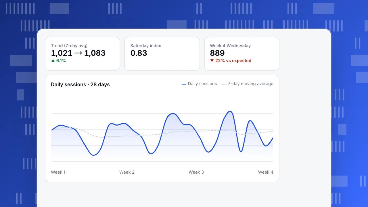
Step 1: remove seasonality to see the trend. A 7-day moving average smooths out the weekly pattern: 1,021 at the end of week 1, 1,047 after week 2, 1,083 after week 3. Traffic is growing steadily, roughly 3% a week.
Step 2: measure the seasonality. Dividing each weekday's average by the overall average over the first three weeks gives a weekday index: Monday 1.08, Tuesday 1.11, Wednesday 1.08, Thursday 1.05, Friday 0.95, Saturday 0.83, Sunday 0.90. Saturdays are normally 17% below an average day. A Saturday dip is not news.
Step 3: look for what does not fit. Wednesday of week 4 recorded 889 sessions. The three previous Wednesdays averaged 1,135 with a spread of about ±17. Even allowing for growth, 889 is more than 20% below expectation and far outside normal variation: an anomaly. The cause in this case: a tag manager change removed the analytics script from the pricing pages for one day.
What the simple comparison would have said: week 4 total 7,529 vs week 3 total 7,580, down 0.7%. A one-day 22% drop disappears inside a weekly total. Comparing like with like, same weekday against same weekday, catches it.
Trend (7-day avg)
1,021 → 1,083
▲ 6.1%
Saturday index
0.83
Week 4 Wednesday
889
▼ 22% vs expected
Daily sessions · 28 days
Daily sessions7-day moving averageCore techniques
Smoothing
Moving averages (7-day for daily web data, 4-week for weekly data) remove seasonality and noise to reveal trend. Exponential smoothing weights recent points more heavily and adapts faster.
Seasonal comparison
Compare against the same period in the last cycle: same weekday last week, same week last year. Year-over-year and month-over-month comparisons are the simplest form; see also seasonality.
Decomposition
Split a series into trend, seasonal and residual parts (for example with STL decomposition). Large residuals are where unexplained events live.
Autocorrelation
Today's value is correlated with yesterday's and with last Tuesday's. That violates the independence most basic statistical tests assume, so do not treat 28 days as 28 independent samples when testing a change.
Forecasting
| Method | Idea | Good for |
|---|---|---|
| Seasonal naive | Next Monday = last Monday | A baseline every other method must beat |
| Moving average + growth | Smoothed level × recent growth × weekday index | Quick planning |
| Exponential smoothing (Holt-Winters) | Level, trend and seasonality updated with weights | Stable business metrics |
| ARIMA / SARIMA | Models autocorrelation explicitly | Series with strong dependence |
| Regression with calendar features | Holidays, campaigns, weekdays as variables | When you know the drivers; see regression analysis |
Always compare a forecast with the seasonal naive baseline. If a complex model does not beat "same day last week", it is not adding value.
Common mistakes
- Comparing different weekday mixes. A month with five weekends will look worse than one with four.
- Ignoring tracking changes. New consent banners, script updates and bot filters create steps that look like real changes. Annotate them.
- Over-reading single points. One spike is not a trend; check it against the noise level.
- Fitting straight lines to curves. Growth often slows; extrapolating a linear trend from a strong quarter overshoots.
- Forgetting time zones and partial periods. "Today" is incomplete until midnight in the reporting time zone.
Time series analysis in TapCub
Every TapCub trend chart can be compared with the previous period or the same period last year, aligned by weekday, and annotated with launches and tracking changes; see compare date ranges and add chart annotations. Metric monitors include an anomaly rule that learns the mean and spread of the same weekday over the last 28 days and alerts when a value falls outside the band, the same logic as step 3 above. For deeper modeling, export daily series and use a notebook; see set up traffic alerts.
Sources
- Hyndman, R. J. and Athanasopoulos, G. (2021). Forecasting: Principles and Practice, 3rd ed. OTexts.
- NIST/SEMATECH. e-Handbook: introduction to time series analysis.
- Cleveland, R. B. et al. (1990). STL: a seasonal-trend decomposition procedure based on Loess. Journal of Official Statistics, 6(1).
Was this article helpful?
We use your answers to fix and expand this page.
Couldn’t send. Please try again in a minute.
Thanks for the feedback. We’ll use it to improve this page.You’ve already sent feedback on this page. Thanks.

Data Analyst
Explores traffic sources, conversion funnels, and retention, using clear metric definitions and concrete examples to explain what the numbers mean.