Try it on your own data
Every report in this article is in the free plan. One snippet for web and apps, up to 10 sites.
Start freeRetention modeling fits a curve to a cohort's first months of retention to project how many users stay active later. Avoid a constant monthly rate: users who will leave go early, so it projects too few survivors. In the sample, a model of why the curve flattens landed within 2 users on held-out months while a constant rate missed by 126.
What you will learn
- Month-over-month retention rising (62.0% to 95.4%) means mixed users, so a constant rate fails
- Test every model on months it did not see: total error 258 users (constant), 38 (power law), 3 (shifted beta-geometric)
- Project no further than about twice your observed history: 531 of 2,000 users at month 12, 409 at month 24
What retention modeling does
Retention modeling takes the first few months of a cohort's retention and fits a curve to it, so you can project how many users will still be active at month 12 or 24. The point is not elegance. It is turning "62% came back in month one" into "about 27% will still be here a year from now", which is what a budget, a lifetime-value estimate or a capacity plan needs.
The mistake to avoid is picking the simplest curve. Retention almost never decays at a constant rate, because the users who are going to leave do so early and the rest stay. A model that ignores this projects too few survivors. This article fits three models to one sample cohort, tests them on months the models did not see and projects survivors with the one that holds up. Reading the curve itself is covered on the retention curve page, and building the cohort table in how to do cohort analysis.
Start with the cohort table you already have
Sample data: 2,000 users who signed up in the same month, and how many were active in each month after.
| Month | Active users | Retention from month 0 | Retention from previous month |
|---|---|---|---|
| 0 | 2,000 | 100.0% | — |
| 1 | 1,240 | 62.0% | 62.0% |
| 2 | 1,010 | 50.5% | 81.5% |
| 3 | 880 | 44.0% | 87.1% |
| 4 | 792 | 39.6% | 90.0% |
| 5 | 730 | 36.5% | 92.2% |
| 6 | 684 | 34.2% | 93.7% |
| 7 | 647 | 32.4% | 94.6% |
| 8 | 617 | 30.9% | 95.4% |
Look at the last column. Month-over-month retention climbs from 62.0% to 95.4%. That is the signature of a cohort made of different kinds of users: some leave almost at once, others stay for a long time, and the average improves as the leavers drop out. Any model that assumes one fixed monthly rate will fail on this data. The next three sections show how badly.
To compare models fairly, fit each on months 0 to 5 only and keep months 6, 7 and 8 (684, 647 and 617 users) as a test.
| Month (held out) | Actual | Constant rate | Power law | sBG |
|---|---|---|---|---|
| 6 | 684 | 639 | 694 | 684 |
| 7 | 647 | 560 | 660 | 646 |
| 8 | 617 | 491 | 632 | 615 |
| Total absolute error | 258 | 38 | 3 |
Sample data: models fitted on months 0 to 5 of a 2,000-user cohort, tested on months 6 to 8.
Model 1: constant monthly retention
The simplest model says every user has the same chance of staying each month, so survivors shrink by a fixed fraction: users(t) = users(1) × r^(t−1). Fitting r on months 1 to 5 gives r = (730 ÷ 1,240)^(1/4) = 0.876.
Predictions for months 6 to 8: 639, 560 and 491 users. The actual numbers were 684, 647 and 617. The model is 45, 87 and 126 users too low, and the gap widens every month. It treats the early leavers and the loyal users as one group that leaves at 12.4% a month, so it keeps removing users who are no longer at risk.
Use this model only when you have strong reason to think users are alike, for example a short fixed-length trial where almost everyone behaves the same way.
Model 2: a power-law curve
A power curve, retention(t) = c × t^k, drops fast at first and flattens, which matches the shape better. Fit it by regressing the log of retention on the log of the month for months 1 to 5. On this sample, c = 0.626 and k = −0.329.
Predictions for months 6 to 8: 694, 660 and 632 users, against 684, 647 and 617. The errors are +10, +13 and +15: a little high, and growing slowly. A power curve is a good descriptive tool, and it never reaches zero. That is also its weakness: it has no explanation of why the curve flattens, so it has no way to know when it should flatten more. It also needs a time scale: the curve for month 1 is fixed at c, so the fit depends on which month you call 1.
Model 3: the shifted beta-geometric model
The shifted beta-geometric (sBG) model, from Fader and Hardie, explains the shape instead of fitting it. It assumes each user has their own churn probability p, constant over time, and that p varies across users following a beta distribution with two parameters, α and β. Users with high p leave first; the survivors are the low-p ones, so the cohort's retention rises on its own. The survivor function is:
S(t) = B(α, β + t) ÷ B(α, β), where B is the beta function
The authors note that the model can be implemented in a simple Excel spreadsheet; you find α and β by maximising the likelihood of the observed counts. On months 0 to 5 of the sample cohort the best fit is α = 0.386 and β = 0.632. The average churn probability across users is α ÷ (α + β) = 0.379.
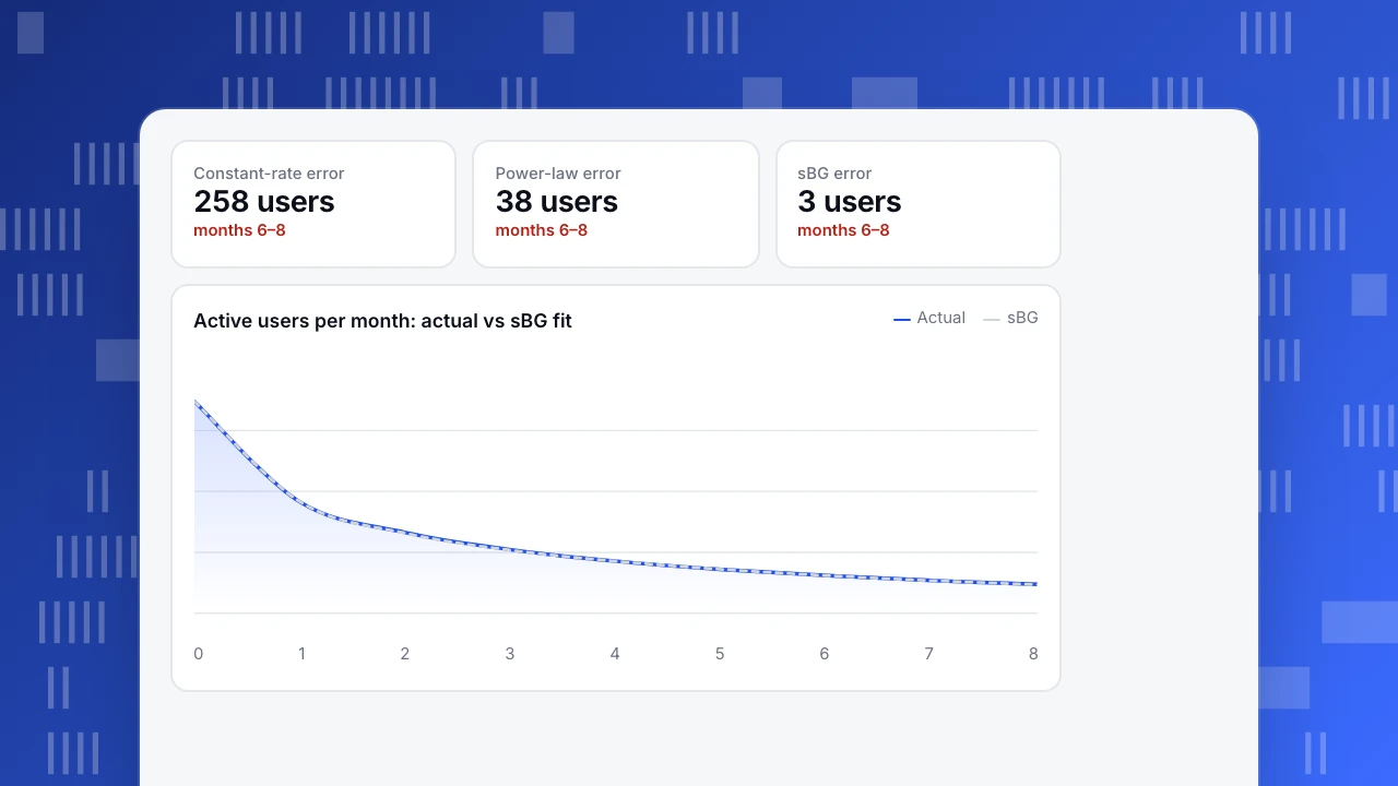
Predictions for months 6 to 8: 684, 646 and 615 users, against 684, 647 and 617. The errors are 0, −1 and −2. The model had never seen those months and still lands within two users.
Compare the three on the months they did not see
| Month (held out) | Actual | Constant rate | Power law | sBG |
|---|---|---|---|---|
| 6 | 684 | 639 | 694 | 684 |
| 7 | 647 | 560 | 660 | 646 |
| 8 | 617 | 491 | 632 | 615 |
| Total absolute error | 258 | 38 | 3 |
The extrapolation gap is bigger than the test gap. Projecting month 12 from the same months 0 to 5: the constant-rate model says 289 users, the power law 553 and sBG 529. A planner who used the first number would expect to keep 14% of the cohort; one who used the third would expect 26%. Holdout testing is what tells you which to believe.
Run this test before you trust any projection: hide the last third of your data, fit on the rest and compare. If the best model is off by more than 5% on the hidden months, do not extrapolate far.
Constant-rate error
258 users
months 6–8
Power-law error
38 users
months 6–8
sBG error
3 users
months 6–8
Active users per month: actual vs sBG fit
ActualsBGProject the survivors
Refit sBG on all nine months: α = 0.383 and β = 0.627. Check the fit is stable, since the months 0 to 5 fit gave 529 at month 12 and the full fit gives 531.
| Month | Projected active users (of 2,000) | Retention |
|---|---|---|
| 12 | 531 | 26.6% |
| 18 | 457 | 22.8% |
| 24 | 409 | 20.5% |
For a new cohort of 5,000 sign-ups with the same behaviour, expect about 1,328 active at month 12 (26.6% of 5,000) and 1,024 at month 24. Round these when you report them, and present a range rather than a point if the decision is large. A good rule: do not project further than about twice the length of your observed data. Nine months of data supports 18 months with confidence; 24 months is an extrapolation.
For lifetime value, add the survivor fractions: summed over months 1 to 12 they give 4.42 active months per sign-up, and over months 1 to 24 they give 7.16. At a sample 20 per active month, that is 88.4 in the first year and 143.1 over two years per sign-up, before costs.
When a retention model breaks
- Mixed cohorts. A cohort that mixes a free-tier signup and a paid signup is two populations; fit each separately.
- Product or pricing changes. A change in month 4 changes the curve after month 4. Fit only the data after it, or mark it.
- Seasonality. Cohorts that start in December and in June can have different shapes. Compare cohorts of the same season.
- Time-varying churn. sBG assumes each user's churn probability does not change. Fader and Hardie's later work adds a duration-dependence extension for the case where it rises or falls over time.
- Revenue is not retention. A user count projection says nothing about spend; model revenue separately.
Build the cohort table in TapCub
The model needs one thing from analytics, the cohort table, and TapCub produces it.
- Set the start and return events. In All-platform analytics › Behavior › Behavior analysis, open retention and pick a start event (for example
signup_completed) and a return event. Leave both empty to mean any activity. - Choose the period. Day, week or month, up to 30 days or 12 weeks or months. For nine months of monthly data, pick month.
- Pick the mode. "Returned on period N exactly" matches the active-users table above. "Returned on N or later" gives a curve that never rises again.
- Read the table. Each row is a cohort with its start date, size, and a count and rate per period; the line below it is the size-weighted average. A period that has not ended yet is empty, not zero, and rates begin at period 1.
- Copy the counts into the model. Take the active-user counts from your oldest full cohort into a spreadsheet or script.
TapCub shows retention; it does not fit curves or forecast survivors. Do that outside, then use the same table next quarter to check the forecast.
FAQ
What is retention modeling?
Retention modeling fits a curve to the observed retention of a cohort so you can project how many users stay active in later periods. It is used for lifetime value, budgets and capacity planning. The model should be tested on months it did not see.
What is the best retention model?
There is no single best model; choose by testing on held-out months. In the sample, a constant-rate model missed month 8 by 126 users, a power law by 15 and the shifted beta-geometric model by 2. The sBG is a strong default when users differ in how likely they are to leave.
How do you project customer retention?
Take a cohort's counts over time, fit a model on the early periods, check it against the later ones you held out, then use it to project further out. Do not project further than about twice your observed history.
Why does retention flatten over time?
Because users differ. The ones most likely to leave go first, so the survivors are increasingly loyal. In the sample, month-over-month retention rises from 62.0% to 95.4% even though no individual user changed.
How many months of data do I need?
Enough to see the curve flatten, usually at least 6 months of a cohort, plus a few more held out for testing. With fewer months, report the projection as a wide range, and refit as more data arrives.
Sources
- Fader, P. S. and Hardie, B. G. S., How to Project Customer Retention, Journal of Interactive Marketing (2007): the shifted beta-geometric model and its spreadsheet implementation. Checked 2026-11-21.
- Fader, P. S., Hardie, B. G. S., Liu, Y., Davin, J. and Steenburgh, T., "How to Project Customer Retention" Revisited: The Role of Duration Dependence, Journal of Interactive Marketing 43 (August 2018), pp. 1–16: the extension for churn that changes over time. Checked 2026-11-21.
Was this article helpful?
We use your answers to fix and expand this page.
Couldn’t send. Please try again in a minute.
Thanks for the feedback. We’ll use it to improve this page.You’ve already sent feedback on this page. Thanks.

Customer Experience Consultant
Writes about live chat, visitor conversations, and self-service, sharing practical ways to make customer communication clearer and more effective.