Try it on your own data
Every report in this article is in the free plan. One snippet for web and apps, up to 10 sites.
Start freeExamples of correlation: weekly emails and sign-ups rise together (r = +0.971), page load time and conversion move in opposite directions (r = −0.958), and blog word count and sign-ups show almost no straight-line link (r = +0.13). This guide gives the raw numbers behind each so you can recompute them, then shows why the same r can hide four different shapes and how to check a coefficient before you trust it.
What you will learn
- r measures straight-line strength from −1 to +1; the sign is direction, r² is the share of variation a line explains, and the labels weak or strong are rules of thumb, not law
- The same r can describe very different data: Anscombe's four datasets all give 0.816, one outlier can drop 0.971 to 0.023, and an exact U-shape gives 0.000
- Before trusting r: plot it, drop the outlier, check n against the threshold (0.632 for 10 points), check the range, and look for a third factor
What does a correlation coefficient actually measure?
The Pearson correlation coefficient, r, measures how closely two numeric variables follow a straight line. It runs from −1 (a perfect downward line) through 0 (no linear pattern) to +1 (a perfect upward line). Compute it by multiplying each pair's distance from the two averages, summing, and dividing by the product of the two spreads:
r = Σ(x − x̄)(y − ȳ) ÷ √[Σ(x − x̄)² × Σ(y − ȳ)²]
Squaring it gives r², the share of the variation in y that a straight line on x accounts for. How to label a value is less settled than the arithmetic. A tutorial in Anesthesia & Analgesia notes that most researchers would call a coefficient below 0.1 negligible and above 0.9 very strong, but that values in between are disputable: whether 0.39 is "weak" and 0.40 is "moderate" is arbitrary. Read r as strength in the context of your question, not against a fixed scale.
Everything below uses ten or eleven points, small enough to recompute in a spreadsheet with CORREL.
What does a positive correlation look like in analytics data?
A positive correlation means the two numbers rise together. Sample data: ten weeks of email volume against sign-ups.
| Week | Emails sent (thousands) | Sign-ups |
|---|---|---|
| 1 | 2 | 31 |
| 2 | 4 | 40 |
| 3 | 5 | 52 |
| 4 | 7 | 55 |
| 5 | 8 | 71 |
| 6 | 10 | 70 |
| 7 | 11 | 88 |
| 8 | 13 | 86 |
| 9 | 14 | 104 |
| 10 | 16 | 99 |
The averages are 9.0 thousand emails and 69.6 sign-ups. Running the formula gives r = +0.971, so r² = 0.943: a straight line on email volume accounts for about 94% of the week-to-week variation in sign-ups. The fitted line is sign-ups ≈ 22.4 + 5.25 × thousands of emails, so each extra 1,000 emails goes with about 5 more sign-ups.
Two cautions. First, "goes with" is not "causes": if you send more email in weeks when launches are happening, the launches could drive both. Second, ten points is few; the correlation needed to clear the 5% two-sided significance bar with n = 10 is |r| ≥ 0.632, and this dataset clears it comfortably. The cause-versus-pattern question has its own page: correlation vs causation.
What does a negative correlation look like?
A negative correlation means one number falls as the other rises. Sample data: ten page templates, with Largest Contentful Paint (LCP, how long the main content takes to appear) against conversion rate.
| Template | LCP (seconds) | Conversion rate (%) |
|---|---|---|
| 1 | 1.2 | 4.1 |
| 2 | 1.6 | 3.6 |
| 3 | 2.0 | 3.9 |
| 4 | 2.4 | 3.2 |
| 5 | 2.8 | 3.4 |
| 6 | 3.2 | 2.8 |
| 7 | 3.6 | 2.9 |
| 8 | 4.0 | 2.4 |
| 9 | 4.5 | 2.5 |
| 10 | 5.0 | 1.8 |
Result: r = −0.958, r² = 0.917. Slower templates convert less, and the line is steep: roughly 0.55 percentage points of conversion lost per extra second. Google's guidance on Core Web Vitals sets 2.5 seconds as the "good" LCP threshold, measured at the 75th percentile of page loads; in this sample, the four templates under 2.5 seconds average 3.7% against 2.6% for the other six.
The negative sign is a direction, not a judgement. Here it is a bad sign for the business; a negative correlation between support tickets and release quality would be a good one. Read the sign against what each axis means.
| Type | Example (sample data) | r | What it tells you |
|---|---|---|---|
| Positive | Emails sent vs sign-ups, 10 weeks | +0.971 | Both rise together; about 5 more sign-ups per 1,000 emails |
| Negative | LCP seconds vs conversion rate, 10 templates | −0.958 | Slower pages convert less; about 0.55 points per second |
| Near zero | Word count vs sign-ups, 10 posts | +0.13 | No straight-line link; below the 0.632 noise threshold |
| Zero, strong link | Price change vs tickets, U-shape | 0.000 | r misses curves; plot before concluding |
Sample data, n = 10 per example (n = 11 for the U-shape); the critical |r| at 5% is 0.632 for n = 10.
What does zero correlation look like?
A coefficient near zero means a straight line on x tells you almost nothing about y. Sample data: ten blog posts, word count against sign-ups attributed to each.
| Post | Words | Sign-ups |
|---|---|---|
| 1 | 600 | 22 |
| 2 | 900 | 35 |
| 3 | 1,200 | 18 |
| 4 | 1,500 | 30 |
| 5 | 1,800 | 41 |
| 6 | 2,100 | 20 |
| 7 | 2,400 | 33 |
| 8 | 2,700 | 19 |
| 9 | 3,000 | 38 |
| 10 | 3,300 | 27 |
Result: r = +0.13, r² = 0.017, well inside the |r| < 0.632 band that n = 10 cannot tell apart from noise. Word count explains under 2% of the variation in sign-ups. The practical reading: length is not what separates the winners here, so look at topic, placement or traffic source instead. Notice what the result does not say: that length never matters anywhere. It says this sample shows no straight-line link.
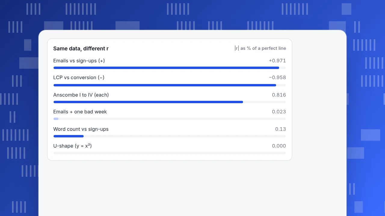
Same data, different r
|r| as % of a perfect lineCan two datasets share the same r and look completely different?
Yes, and the classic proof is Anscombe's quartet, four published datasets of 11 points each (F. J. Anscombe, The American Statistician, 1973). The values below are his, and the r values were recomputed for this article.
| Dataset | Shape when plotted | r |
|---|---|---|
| I | Noisy upward line | 0.816 |
| II | Smooth curve that rises, peaks and falls | 0.816 |
| III | Perfect line plus one outlier (x = 13, y = 12.74) | 0.816 |
| IV | All points at x = 8 except one at x = 19 | 0.816 |
All four also share x̄ = 9.0, ȳ ≈ 7.5 and the fitted line y = 3 + 0.5x. The number is identical; the stories are four different ones. Dataset III shows the outlier effect numerically: drop the one point at x = 13 and r jumps from 0.816 to 1.000. Dataset IV is the opposite: the whole correlation rests on one point, and removing it leaves x constant, so r cannot even be calculated.
The same fragility shows up in everyday analytics data. Take the email sample from earlier and add one eleventh week with 30,000 emails and only 20 sign-ups (a send that hit a broken landing page). The correlation collapses from 0.971 to 0.023. One bad week erased a clear pattern, which is exactly why you chart before you quote the number.
Can r be zero when there is a strong relationship?
Yes, because r only detects straight lines. Sample data: price changes from −5% to +5% in one-point steps, against support tickets that rise with the size of the change in either direction (tickets = change²: 25, 16, 9, 4, 1, 0, 1, 4, 9, 16, 25).
The relationship is exact (every ticket count is determined by the price change), yet r = 0.000, because the left half slopes down and the right half slopes up and the two cancel. The same tutorial that discusses the thresholds warns that correlation "fails to adequately describe nonlinear or nonmonotonic relationships" and recommends always inspecting the scatter plot. For curved but one-directional patterns (always rising, flattening out), a rank-based coefficient such as Spearman's is better; for U-shapes like this one, bucket x and compare group averages.
How do you check an r value before you trust it?
Run these five checks in order; stop at the first one that fails.
- Plot first. A scatter plot (see scatter plot) shows curves, clusters and outliers that one number hides. Anscombe's four datasets are indistinguishable without it.
- Test the outlier. Recompute without the most extreme point. If r moves by more than about 0.2, report both values.
- Check n against the threshold. With 10 points you need |r| ≥ 0.632 to be distinguishable from noise at the 5% level; with 30 points, about 0.361. A big r on a handful of points proves little.
- Check the range. A narrow slice of x (only template pages under 2 seconds) produces a weaker r than the full range shows.
- Ask what else moves both. Launches, seasonality or a traffic source can drive both variables. If you can split the data by that factor, do; if you cannot, say so.
The coefficient also assumes each pair is independent. Ten daily readings from one visitor, or 30 days of one metric where each day depends on the last, break that assumption and make r look more convincing than it is.
How do you work with correlation in TapCub?
Suppose you want to run the email sample above on your own data. TapCub supplies the counts; the coefficient itself you compute outside. TapCub does not calculate correlation coefficients or draw scatter plots.
- Open All-platform analytics › Behavior › Behavior analysis, add the two measurements you want to compare (for example a campaign click event and your sign-up event), and set the granularity to day or week. The Trend tab shows both series over the same range.
- Switch to the Table tab and export the result as CSV.
- In a spreadsheet, put the two columns side by side and use
CORRELand a scatter chart. Run the five checks above, including the outlier test. - Mark the unusual week. If it was a launch or an outage, add it under Configuration › Annotations so the next reader of the chart sees why it is there.
- Before you believe the pattern, break the same measurements down by source or device in the same report and see whether it holds in each group; a pattern that holds only in one group is a pooling effect, not a general relationship.
FAQ
What is an example of a positive correlation?
Weekly email volume and sign-ups in the sample above: both rise together, r = +0.971. Familiar everyday examples are height and weight, or hours studied and test scores. A positive correlation says nothing about which variable, if either, drives the other.
What is an example of a negative correlation?
Page load time and conversion rate: in the ten-template sample, r = −0.958, so slower pages convert less. Elevation and air temperature is another familiar one. The negative sign only means the variables move in opposite directions.
What is an example of zero correlation?
Word count and sign-ups across ten blog posts in the sample (r = +0.13). Zero correlation means no straight-line pattern, not no relationship: price change against support tickets has r = 0.000 despite an exact U-shaped link.
How strong is a correlation of 0.5?
Moderate by most rules of thumb, and it explains 25% of the variation (r² = 0.25). But the cutoffs are arbitrary, so state the number and its r² rather than only the label, and check how many points sit behind it.
Does correlation prove causation?
No. A correlation shows two variables move together; it does not show that one causes the other, because a third factor or reverse direction can produce the same pattern. Controlled experiments, or careful stratification, are the way to test cause.
Sources
- Schober P, Boer C, Schwarte LA. Correlation Coefficients: Appropriate Use and Interpretation. Anesthesia & Analgesia, 126(5), May 2018 — thresholds, outliers, nonlinear relationships. Verified 2026-11-20.
- Anscombe FJ. Graphs in Statistical Analysis. The American Statistician, 27(1), 1973 — the four datasets; values checked against Duke STA 290 lecture notes on 2026-11-20.
- Google. Web Vitals — LCP "good" threshold of 2.5 seconds at the 75th percentile. Verified 2026-11-20.
Was this article helpful?
We use your answers to fix and expand this page.
Couldn’t send. Please try again in a minute.
Thanks for the feedback. We’ll use it to improve this page.You’ve already sent feedback on this page. Thanks.

Data Engineer
Writes about event design, data quality, and collection workflows, with verifiable implementation methods for reliable analytics.