Try it on your own data
Every report in this article is in the free plan. One snippet for web and apps, up to 10 sites.
Start freeAggregation means reducing many records to one value with a function such as a sum, average, count or maximum. It makes data readable, but it throws detail away, so the grain and the step at which you aggregate decide whether you can still find the problem. Below: what each function hides, three traps with worked numbers, and how to choose.
What you will learn
- Never average ratios: add the numerators and the denominators, then divide (4.67% in the example, not 6.25%)
- Before trusting a total, split it by device or channel; a winner can flip when groups are combined
- Keep a grain fine enough to show one bad day, and recompute distinct counts instead of adding daily ones
What aggregation means
To aggregate is to take many records and reduce them to one value with a function: add them up, average them, count them, take the largest. "Aggregation" is the act, "aggregating" is doing it, and "aggregated data" is the result: one row that stands in for many. Ten orders become "total revenue: $412". Two million page views become "visitors per day".
The word is also used for a second job, gathering data from several places into one store. That is closer to data integration, and the data aggregation glossary entry covers the vocabulary. This guide is about the first sense, summarizing rows, and about what that summary loses.
The loss is the point. A summary is useful exactly because it throws detail away, and it is risky for the same reason. Which detail you discard, and at which step, decides whether you can still find the problem afterwards. The rest of this guide is a way to choose on purpose.
The common aggregate functions and what each one hides
Almost every report is built from six functions. Each answers one question and hides something specific.
| Function | Answers | Good for | What it hides |
|---|---|---|---|
| COUNT | How many records? | Orders, sessions, errors | Whether they belong to few people or many |
| COUNT DISTINCT | How many different ones? | Visitors, customers | Who came back and how often |
| SUM | How much in total? | Revenue, page views | Whether it came from one big item or a thousand small ones |
| AVERAGE (mean) | What is a typical value? | Order value, time on page | Outliers and the shape of the spread |
| MEDIAN / percentile | What is the middle, or the slow tail? | Durations, load times | Anything above or below the point you picked |
| MIN / MAX | What is the extreme? | Peak load, first and last date | How often it happens |
Two details trip people up in practice. In SQL, COUNT(*) counts rows including ones with missing values, while COUNT(column), SUM, AVG, MIN and MAX skip missing values, and, except for COUNT, return nothing rather than zero when no rows match, as the PostgreSQL manual documents. So "average revenue per customer" quietly changes meaning if customers with missing revenue are dropped instead of counted as zero. State which one you did.
A worked example: simple average versus weighted average
Sample data: four channels sent traffic to a store last month.
| Channel | Sessions | Orders | Conversion rate |
|---|---|---|---|
| 500 | 60 | 60 ÷ 500 = 12.0% | |
| Search | 3,000 | 120 | 120 ÷ 3,000 = 4.0% |
| Social | 1,500 | 30 | 30 ÷ 1,500 = 2.0% |
| Direct | 1,000 | 70 | 70 ÷ 1,000 = 7.0% |
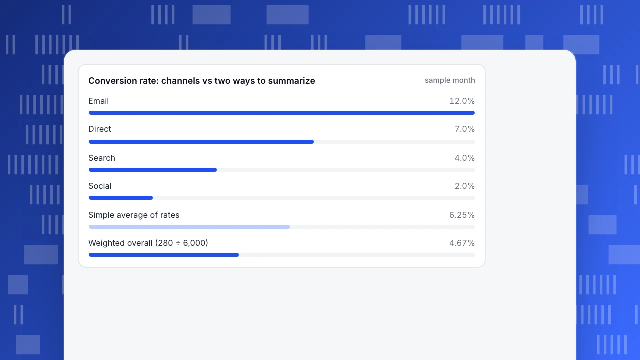
A quick summary averages the four rates: (12.0 + 4.0 + 2.0 + 7.0) ÷ 4 = 6.25%. That treats the 500-session email channel as equal to the 3,000-session search channel, so the small, high-converting channel pulls the figure up.
The honest overall rate adds up the orders and the sessions first, then divides: (60 + 120 + 30 + 70) ÷ (500 + 3,000 + 1,500 + 1,000) = 280 ÷ 6,000 = 4.67%. This is a weighted average, where each channel counts in proportion to its sessions. The two figures differ by 6.25 − 4.67 = 1.58 percentage points, so the simple average overstates conversion by about a third (1.58 ÷ 4.67 = 34%).
The rule that falls out: never average ratios; sum the numerators and the denominators, then divide. It holds for conversion rate, bounce rate, click-through rate and any other "x per y" figure.
Conversion rate: channels vs two ways to summarize
sample monthTrap 1: an average hides the distribution
An average describes a typical value only when the values cluster. When one very large value sits among small ones, it drags the mean away from where most of the data is.
Sample data: ten sessions, in seconds: 12, 15, 18, 20, 22, 25, 30, 35, 40 and 1,800 (a tab left open overnight).
- Mean: (12 + 15 + 18 + 20 + 22 + 25 + 30 + 35 + 40 + 1,800) ÷ 10 = 2,017 ÷ 10 = 201.7 seconds.
- Median: the middle of ten values is the average of the fifth and sixth, (22 + 25) ÷ 2 = 23.5 seconds.
A report that says "average session: 3 minutes 22 seconds" describes no session in the sample. Nine of the ten lasted under a minute. The NIST/SEMATECH Engineering Statistics Handbook states the general principle: the mean is sensitive to extreme values and the median is not, so for data with extreme tails the median is generally the better estimate of the centre. The full comparison is in mean vs median.
Fix: for anything that has a long tail (durations, load times, order values), report the median and a high percentile, such as P90, next to the mean, or instead of it.
Trap 2: Simpson's paradox, when the total says the opposite of every group
Sometimes a trend that holds inside every group reverses in the combined total. This is Simpson's paradox. The classic case is the 1973 Berkeley graduate admissions data analysed by Bickel, Hammel and O'Connell (1975): men were admitted at a higher rate overall, yet no department showed bias against women, because women applied more to the departments with lower admission rates.
Sample data: you test page A against page B. Both pages are shown to 1,000 visitors, but traffic mix differs.
| Page | Mobile visits | Mobile orders | Desktop visits | Desktop orders | Overall |
|---|---|---|---|---|---|
| A | 100 | 5 (5.0%) | 900 | 180 (20.0%) | 185 ÷ 1,000 = 18.5% |
| B | 600 | 42 (7.0%) | 400 | 88 (22.0%) | 130 ÷ 1,000 = 13.0% |
Page B wins on mobile (7.0% versus 5.0%) and on desktop (22.0% versus 20.0%), yet loses overall (13.0% versus 18.5%). Nothing is miscalculated. Page B simply received mostly mobile visitors, who convert less on both pages, so its overall rate is dragged down by the mix, not by the page.
Fix: before declaring a winner from a summary number, split it by the dimension that most plausibly changes behavior (device, channel, country, new versus returning) and check whether the direction holds in each group. If it flips, the total is measuring the mix.
Trap 3: grain that is too coarse, and totals that do not add
Two further problems come from how far you aggregate.
A coarse grain hides an event. Sample data: a store gets 1,000 sessions a day. Daily orders over a week are 40, 41, 40, 0, 42, 41 and 40. On day four the checkout was broken. The weekly view says 244 orders ÷ 7,000 sessions = 3.49%. Normal days convert at 244 ÷ 6,000 = 4.07%. The weekly figure looks about 14% worse than usual, which suggests a gradual slide, while the truth is one day of zero and six normal days. Only the daily grain shows it. This is the question of data granularity: the level of detail at which each row is kept.
Some totals cannot be added up. Counts of events and sums of amounts add across days. Counts of distinct people do not. Sample data: daily unique visitors of 100, 110 and 90 add up to 300, but many people came on more than one day, so the number of different people across the three days might be only 180. Summing daily uniques counts a returning person once per day. The same applies to averaging averages, such as the mean of daily means when days have different traffic.
Fix: keep a grain fine enough to show a single bad day, and for distinct counts compute the unique number over the whole period from the underlying records instead of adding daily figures.
| Trap | What you see | Check |
|---|---|---|
| Averaging ratios | Overall rate too high (6.25% vs 4.67%) | Sum numerators and denominators, then divide |
| Mean with outliers | A typical value no record matches (201.7 s vs 23.5 s median) | Report the median and P90 |
| Mixed groups | Winner flips in the total (B wins both groups, loses overall) | Split by device, channel or country |
| Coarse grain | One broken day looks like a slide (3.49% vs 4.07%) | Keep a daily or hourly view |
| Summed distinct counts | People counted once per day (300 vs maybe 180) | Compute uniques over the whole period |
Each row is one worked example in this article.
How to choose what to aggregate and when
Use five questions, in order. Each one maps to a rule.
| Question | Rule |
|---|---|
| What decision will this number feed? | Pick the grain at which someone could act: hourly for an outage, weekly for a trend, monthly for a budget. |
| How fast does the thing change? | Aggregate at the speed of change. Anything that can break in a day needs a daily or hourly view. |
| How many records fall in each bucket? | If a bucket holds only a handful of records, widen it. A rate from 10 sessions swings wildly. |
| Is the metric additive? | Counts and sums add. Distinct counts and ratios do not; recompute them from the underlying records. |
| Can you get back to the detail? | Keep the raw records for as long as your retention rules allow, and aggregate when you read. Store only aggregates when you do not need the detail, or must not keep it. |
The last row has a privacy side. Storing only summaries limits what could leak, but a summary of a very small group can still point to a person, so decide on a minimum group size before showing a breakdown.
How to read aggregated numbers in TapCub
Take the channel table from the worked example and see how TapCub shows the same figures.
- Pick the grain deliberately. Web analytics › Reports shows one row per time bucket, and the grain can be hour, day, week, month or year; hourly view is limited to seven days. Use the daily grain to catch a day like day four of the checkout example, then widen to weeks for the trend.
- Trust the totals row for ratios. In that report the total row sums counts across rows, and ratios and averages are computed by adding numerators and denominators separately and then dividing. That is the weighted calculation from the example (280 ÷ 6,000), not an average of daily rates.
- Remember that visitor totals add across days. The visitors total is the sum of the days, so a person who came three days counts three times. For ranges of up to 93 days the table also shows the number of distinct visitors across the whole range; use that one when you mean "how many different people". With a daily-rotating salt, as in the anonymous aggregate tier or strict mode, the same person cannot be matched across days at all.
- Split before you conclude. Break the same period down in Web analytics › Sources and check that the direction holds per channel, as in the Simpson's paradox example.
- Choose the measure that fits the shape. In All-platform analytics › Behavior › Metrics & SQL you can define a metric as an event plus an aggregation, such as unique people, average per person, median or P90, so a duration report need not rely on the mean.
TapCub does not tell you whether your aggregate is the right one for the decision; the choice of grain and measure stays with you.
FAQ
What does aggregating data mean?
Aggregating data means combining many records into a single summary value, such as a sum, average, count or maximum. A table of 6,000 sessions becomes one conversion rate. Aggregation makes data readable and storable, but it removes the detail needed to see outliers, groups and single bad days.
What is aggregated data?
Aggregated data is the output of aggregating: a figure or a table of figures that stands for many underlying records, such as daily visitors, monthly revenue by channel or a single average. It is the opposite of raw, record-level data, which keeps every individual row.
Is aggregated data anonymous?
Not automatically. A total across thousands of people reveals little about any one of them, but a breakdown that ends up with a bucket of two or three people can point to an individual. Set a minimum group size before publishing a breakdown, and treat small buckets with care.
What is the difference between aggregation and averaging?
Averaging is one kind of aggregation. Aggregation also includes counting, summing, taking minimums and maximums, and computing medians or percentiles. When you average rates, the result can mislead; sum the numerators and denominators and divide instead, as in the weighted example above.
When should you not aggregate?
Do not aggregate away the grain you need to investigate a problem. If you may need to find one bad day, one bad device or one bad campaign, keep records at that level and aggregate when you read the report, not when you store it.
Sources
Was this article helpful?
We use your answers to fix and expand this page.
Couldn’t send. Please try again in a minute.
Thanks for the feedback. We’ll use it to improve this page.You’ve already sent feedback on this page. Thanks.

Data Analyst
Explores traffic sources, conversion funnels, and retention, using clear metric definitions and concrete examples to explain what the numbers mean.